Native Hartree-Fock
Before a molecule's electronic-structure problem can become a qubit Hamiltonian, its
integrals (overlap, kinetic, nuclear-attraction, electron-repulsion) have to be
computed and a Hartree-Fock mean-field calculation run to get a reference orbital
basis. dense_evolution.native_hf is a from-scratch, JAX-vectorized engine for that
step -- covers any element basis_set_exchange has STO-3G data for, not just the small
H-Ne table PennyLane's own bundled solver ships.
The hf extra installs basis_set_exchange, which supplies the basis-set data. Step 1
also builds a PennyLane Hamiltonian, so it needs pip install dense-evolution[pennylane],
which includes the same package.
Step 1. A real molecule's qubit Hamiltonian
import numpy as np
from dense_evolution.native_hf.bridge import build_qubit_hamiltonian

geometry = np.array([[0.0, 0.0, 0.0], [0.0, 0.0, 0.7414]])
H, n_qubits, hf_result = build_qubit_hamiltonian([1, 1], geometry, n_electrons=2)

n_qubits, hf_result.converged, hf_result.n_iterations, hf_result.total_energy
build_qubit_hamiltonian(atomic_numbers, geometry_angstrom, n_electrons) runs the full
pipeline -- Obara-Saika integrals, then Hartree-Fock self-consistent-field iteration
(run_scf, DIIS-accelerated) -- for H2 (two protons, atomic number 1, 0.7414 Angstrom
apart, the real equilibrium bond length) in the default STO-3G minimal basis. It
converged in 3 iterations to a mean-field energy of -1.1167 Ha. H is a qml.Hamiltonian -- the
converged result still goes through PennyLane's own fermionic_observable +
jordan_wigner for the qubit mapping, since that stage was already fast and
well-tested; this module only replaces the slow integral/SCF stage.
Step 2. Hartree-Fock is a mean-field approximation -- how far off?
import dense_evolution as de

coeffs, ops = H.terms()
terms = []
for coeff, op in zip(coeffs, ops):
    pauli = {}
    for factor in (op.operands if hasattr(op, 'operands') else [op]):
        if factor.name != 'Identity':
            pauli[int(factor.wires[0])] = factor.name[-1]
    terms.append((float(np.real(complex(coeff))), pauli))

H_dense = de.pauli_hamiltonian_to_matrix(terms, n_qubits)
float(np.min(np.linalg.eigvalsh(H_dense)))
Converting H's Pauli terms to pauli_hamiltonian_to_matrix's format
and exactly diagonalizing gives -1.1373 Ha -- lower than Step 1's Hartree-Fock energy
by about 0.02 Ha, the real electron-correlation energy Hartree-Fock's single-Slater-
determinant approximation misses entirely. At only 4 qubits, exact diagonalization is
easy; that gap is exactly what a real VQE ansatz beyond a bare Hartree-Fock reference
state is trying to close for larger, classically-intractable molecules.
Step 3. Large mixed-basis molecules: the optional libcint bridge
import numpy as np
from dense_evolution.native_hf.basis import build_molecule_shells
from dense_evolution.native_hf.assembly import build_overlap_matrix, build_core_hamiltonian
from dense_evolution.native_hf.libcint_bridge import build_repulsion_tensor_libcint
from dense_evolution.native_hf.scf import run_scf

geometry = np.array([[0.0, 0.0, 0.0]])
shells = build_molecule_shells([10], geometry, "6-31g*")
S = build_overlap_matrix(shells)
H_core = build_core_hamiltonian(shells, [10.0], geometry)
V = build_repulsion_tensor_libcint([10], geometry, "6-31g*")

result = run_scf(S, H_core, V, 10, [10.0], geometry)
result.converged, result.total_energy
Step 1's molecule only needed s functions, so build_repulsion_tensor (the
default, pure-JAX path) was already fast. A basis mixing s, p, and d shells
-- like 6-31g* on neon here -- costs much more with the default path: the
underlying JIT compiles one program per distinct shell-quartet shape it
meets, and a mixed basis needs dozens of them. build_repulsion_tensor_libcint
computes the identical tensor through
libcint instead -- a mature C library with no per-basis compile cost at
all -- and is a drop-in replacement everywhere build_repulsion_tensor's
output was used (S and H_core above still come from native_hf itself).
libcint ships inside the dense-evolution wheels for Windows, macOS and Linux,
so pip install dense-evolution is enough. On neon in 6-31g* the tensor takes 0.013 s; on ethanol
(57 basis functions) 0.32 s, against 0.50 s for PySCF on the same Linux machine.
Step 4. Diagnosing a stubborn SCF: energy_history
from dense_evolution.native_hf.scf import diagnose_convergence

result = run_scf(S, H_core, repulsion, n_electrons, nuclear_charges, geometry_bohr)
diagnosis = diagnose_convergence(result)
print(diagnosis["anomaly_fraction_hampel"])
run_scf already computes the electronic energy at every iteration --
HFResult.energy_history now keeps that trace instead of throwing it
away (shape (max_iterations,), NaN past n_iterations).
diagnose_convergence runs Dense-Armor's own Hampel filter and Tukey
fences (dense_evolution.utility.robust_filters -- the sister project's
anomaly detectors, validated with 0 false positives on real H2
dissociation-curve chemistry) over that trace, instead of trusting the
final converged flag in isolation.
Measured, not assumed: a real 28-heavy-atom CASMI26 fragment (this
module's own level_shift docstring) that fails to converge at
level_shift=0.0 has its 200-iteration electronic-energy trace flagged
19-24% anomalous (Hampel/Tukey); the identical fragment, fixed with
level_shift=0.5 (converges in 55 iterations), flags only ~4% --
background noise, not a false-alarm storm. Needs the armor extra
(pip install dense-evolution[armor]); dense_armor is not a hard
dependency of this module.
Step 5. Energy as a function of the atoms' positions
Step 1 gives the energy of one molecule at one fixed geometry. But the interesting questions are about change: how much does the energy rise if the two atoms are pulled apart? What force does each nucleus feel? Where is the equilibrium bond length? All of these need the energy as a function of the atomic positions, plus its gradient.
import numpy as np
from dense_evolution.native_hf.differentiable import build_energy_fn

geom = np.array([[0.0, 0.0, 0.0], [0.0, 0.0, 1.4011]])

energy_fn = build_energy_fn(
    atomic_numbers=[1, 1],
    nuclear_charges=[1.0, 1.0],
    n_electrons=2,
    basis_name="sto-3g",
    reference_geometry_bohr=geom,
)

energy_fn(geom)
geom is the two hydrogen atoms at the experimental bond length, in Bohr
(1.4011 Bohr is 0.7414 Å, the geometry of Step 1; the energy matches
Step 1's up to that rounding). build_energy_fn returns a plain function
geometry_bohr -> total energy in Hartree, differentiable end-to-end with
jax.grad, so jax.grad(energy_fn) gives the force on each nucleus
directly. Here it is ±0.029 Hartree/Bohr along the bond, not zero: with
the STO-3G basis the energy minimum is slightly shorter than the
experimental bond length.
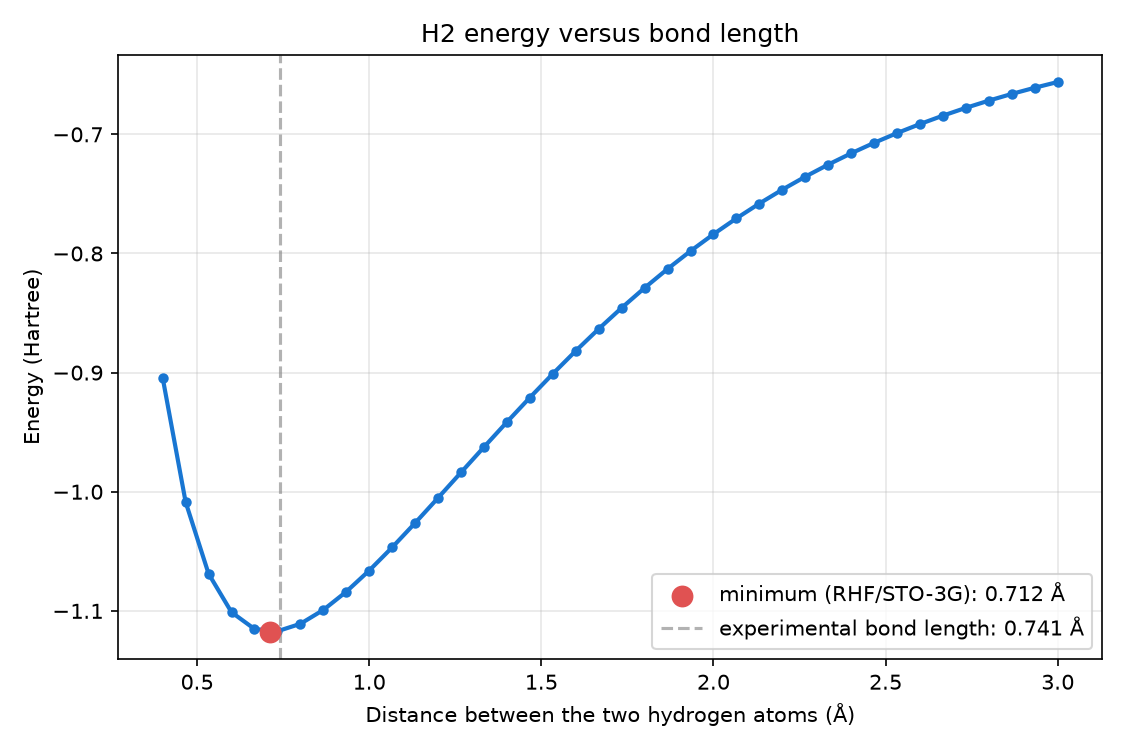
The curve this engine produces when the two hydrogen atoms are moved apart
and the energy is computed at each distance. Pull them away and the energy
rises toward two separate atoms; push them together and it rises because
the nuclei repel each other. With RHF/STO-3G the minimum sits at 0.712 Å,
-1.117506 Hartree; the experimental bond length is 0.741 Å. The gap is
the basis set and the mean-field approximation, not the integrals.
Step 6. Unpaired electrons: UHF and ROHF
Every molecule so far has its electrons in pairs. A radical such as OH has 9 electrons, so one is left alone; transition-metal atoms (Cr, Ti, V) can have several. RHF puts both electrons of a pair in the same orbital, which cannot describe an unpaired one. UHF lets the two spins have different orbitals; ROHF keeps the pairs together and only the unpaired electrons apart.
import numpy as np
from dense_evolution.native_hf.assembly import build_core_hamiltonian, build_overlap_matrix, build_repulsion_tensor
from dense_evolution.native_hf.basis import build_molecule_shells
from dense_evolution.native_hf.scf import run_cuhf, run_uhf

geom = np.array([[0.0, 0.0, 0.0], [0.0, 0.0, 1.83]])
shells = build_molecule_shells([8, 1], geom, "sto-3g")
S, H, V = build_overlap_matrix(shells), build_core_hamiltonian(shells, [8.0, 1.0], geom), build_repulsion_tensor(shells)

uhf = run_uhf(S, H, V, 9, [8.0, 1.0], geom)
rohf = run_cuhf(S, H, V, 9, [8.0, 1.0], geom)
print(uhf.total_energy, uhf.spin_squared)
print(rohf.total_energy, rohf.spin_squared)
OH is an oxygen and a hydrogen 1.83 Bohr apart. n_unpaired defaults to
9 % 2 = 1, so there are 5 alpha and 4 beta electrons. spin_squared is
⟨S²⟩: a single unpaired electron should give exactly 0.75. UHF finds a
slightly lower energy but ⟨S²⟩ = 0.7532, a small spin contamination
from mixing in higher spin states. run_cuhf is ROHF written as a
constrained UHF (Tsuchimochi & Scuseria, arXiv:1008.1607): ⟨S²⟩ = 0.75
exactly, at an energy 1.1 mHartree higher. With no unpaired electrons
both give the RHF energy. For an energy-versus-distance scan, pass the
previous point's orbital_coefficients_alpha / _beta as C_alpha_init
/ C_beta_init, so every point stays in the same SCF solution.
Step 7. A real open-shell transition metal: the Cr-O curve
Step 6 introduced UHF and ROHF (as constrained UHF) on OH and O2. The test case that motivated that work is the Cr-O dimer: neutral, an open-shell 3d metal bound to oxygen, 32 electrons, where a single closed-shell Slater determinant is the wrong ansatz and the RHF SCF oscillates between local minima at adjacent geometries. This is Dense-Evolution issue #358.
The setup is the issue's own. Cr-O dimer, 3-21g basis,
32 electrons, R from 1.6 to 2.4 Å along the x axis, ERI tensor from
build_repulsion_tensor_libcint, SCF from run_uhf / run_cuhf.
Warm start: the previous point's converged
orbital_coefficients_alpha / orbital_coefficients_beta seed the
next point's C_alpha_init / C_beta_init, so the SCF stays in the
same local minimum across the whole curve. First point uses the
core-Hamiltonian guess.
RHF reference (issue #358, level_shift=0.0):
k = -22 Ha/A^2      (impossible sign for a bound diatomic)
energy jumps ~0.2 Ha between adjacent geometries
Best spin state found: n_unpaired = 6, CUHF, at
R_e = 1.9112 Å, E(R_e) = -1112.709156 Ha, k = 0.8454 Ha/Ų.
R (A) E (Ha) dE to prev conv iter <S^2>
1.600 -1112.64892582 --- True 36 12.0000000000 1.657 -1112.67345374 -2.452791e-02 True 27 12.0000000000 1.714 -1112.69015513 -1.670140e-02 True 24 12.0000000000 1.771 -1112.70074104 -1.058591e-02 True 28 12.0000000000 1.829 -1112.70660382 -5.862775e-03 True 27 12.0000000000 1.886 -1112.70886625 -2.262434e-03 True 27 12.0000000000 1.943 -1112.70842308 +4.431677e-04 True 24 12.0000000000 2.000 -1112.70597669 +2.446389e-03 True 24 12.0000000000 2.057 -1112.70206892 +3.907772e-03 True 24 12.0000000000 2.114 -1112.69711018 +4.958745e-03 True 24 12.0000000000 2.171 -1112.69140609 +5.704084e-03 True 25 12.0000000000 2.229 -1112.68518136 +6.224732e-03 True 25 12.0000000000 2.286 -1112.67860023 +6.581131e-03 True 25 12.0000000000 2.343 -1112.67178336 +6.816871e-03 True 25 12.0000000000 2.400 -1112.66482098 +6.962378e-03 True 25 12.0000000000
Max neighbour jump along the curve:
max |E(R_i) - E(R_(i+1))| = 0.024528 Ha
against the issue's RHF table, where adjacent-geometry jumps reached
~0.2 Ha. Parabola fit on the five points around the minimum:
R_e      = 1.911155 A
E(R_e)   = -1112.70915634 Ha
k = 2*a2 = 0.845422 Ha/A^2
k > 0 and of the expected order of magnitude for a metal–oxygen
bond; the RHF fit gave k = -22 Ha/Ų, the wrong sign and no bound
state.
All three spin states tested, at their respective minima:
| method | n_unpaired | S(S+1) | E_min (Ha) | R(E_min) (Å) |
|---|---|---|---|---|
| UHF | 2 | 2 | -1112.515060 | 1.6571 |
| UHF | 4 | 6 | -1112.694485 | 1.7714 |
| UHF | 6 | 12 | -1112.680050 | 1.8286 |
| CUHF | 2 | 2 | -1112.432516 | 1.6571 |
| CUHF | 4 | 6 | -1112.608024 | 1.6000 |
| CUHF | 6 | 12 | -1112.708866 | 1.8857 |
CUHF keeps <S^2> = S(S+1) to 3.55e-14 across the whole
n_unpaired = 6 curve; UHF contaminates by up to 3.82e-03 on the
same state (range [12.001745, 12.003817]). For n_unpaired = 6 the
UHF minimum (-1112.680050 Ha) lies above the CUHF one
(-1112.708866 Ha): UHF is the less constrained method, so its true
minimum cannot be higher, and the warm-started UHF scan has settled in
a higher local minimum. For n_unpaired = 2 and 4 the CUHF minima
sit at the edge of the grid (1.60–1.66 Å), so they are not interior
minima of the scan.
All five assertions passed: every point converged, k > 0, CUHF
<S^2> = S(S+1) to 1e-8, max neighbour jump below 0.05 Ha.
What is still open. DFT+U and CASSCF are the standard methods for
3d/4f transition-metal oxides and remain unimplemented. UHF and CUHF
unblock the E(R) curve — a smooth curve now exists, and the parabola
fit gives a physically meaningful k > 0 — but neither captures
dynamic correlation, and neither accounts for localization on the
metal centre. The values of R_e and k above should be read as
method-consistent, not as benchmark numbers: Hartree-Fock with a small
basis is known to favour high-spin states in transition-metal oxides,
and the spin state and bond length found here have not been compared
with a spectroscopic reference for CrO. Closing that gap is a
larger change to the codebase, as the issue itself notes.
To reproduce: python scripts/simulator_infrastructure/cr_o_open_shell_curve.py in Dense-Evolution-Discovery (about 2 minutes on a laptop CPU with libcint).
Step 8. Forces on an open-shell molecule
Step 5 gave the force on each nucleus of H2. The same build_energy_fn takes
method="uhf" or method="cuhf", so forces work for molecules with unpaired electrons too.
import numpy as np
import jax
from dense_evolution.native_hf.differentiable import build_energy_fn

geom = np.array([[0.0, 0.0, 0.0], [0.0, 0.0, 1.83]])

energy_fn = build_energy_fn(
    atomic_numbers=[8, 1], nuclear_charges=[8.0, 1.0], n_electrons=9,
    basis_name="sto-3g", reference_geometry_bohr=geom,
    method="uhf", n_unpaired=1,
)

print(float(energy_fn(geom)))
print(float(jax.grad(energy_fn)(geom)[1, 2]))
The energy is the UHF energy of OH from Step 6. The second number is dE/dz of the hydrogen
in Hartree/Bohr; a central finite difference of the same energy (step 1e-4 Bohr) gives
-0.0579597653, a difference of 4e-9. The gradient is analytic: at the converged SCF the
energy is stationary, so only the explicit dependence of the integrals counts, with the
spin-resolved energy-weighted density W_s = C_s,occ diag(eps_s,occ) C_s,occ^T for each spin
(Lehtola, Blockhuys & Van Alsenoy, arXiv:1912.12029). For method="cuhf" the constrained
Fock matrices differ from the UHF ones only in the core-virtual block of the natural-orbital
basis, which does not touch the occupied orbitals, so the same W_s applies; the tests check
it against finite differences on OH and O2.
Details
Why this module exists: PennyLane's own differentiable Hartree-Fock solver
(qml.qchem, method="dhf") builds the same integrals through a Python-level loop
wrapped in its autograd-tracing numpy layer -- correct, but profiled directly at 482 of
483 total seconds for Si2/STO-3G, almost entirely per-scalar-op tracer overhead rather
than real FLOPs. This module batches each shell-pair/quartet with jax.lax.scan/
jax.vmap and compiles with jax.jit instead.
Elements beyond PennyLane's table: basis-set parameters come from
basis_set_exchange, so any
element it has STO-3G data for is reachable -- an element needing d-orbitals or higher
(e.g. Fe) fails with a clear NotImplementedError naming the real limitation, not a
silent wrong energy for an incomplete basis.
Verified against an independent implementation: element-wise against
lowdanie/hartree-fock-solver
("slaterform", Apache-2.0, studied as a reference for structuring the Obara-Saika
recursion with jax.lax.scan -- no source code copied) to machine precision on
individual integrals. The original Si2/STO-3G full-SCF-energy cross-check against
slaterform predates the DIIS/Si2-convergence fix below and has not been re-run against
the corrected energy -- the per-integral cross-check is unaffected (integrals don't
depend on how the SCF loop converges), but the end-to-end Si2 number should be treated
as not yet re-verified against this independent reference. Algorithm background also
drawn from PennyLane's own white paper (Delgado et al., "Differentiable quantum
computational chemistry with PennyLane", arXiv:2111.09967).
The libcint bridge's AO conventions: libcint_bridge.py builds libcint's
atm/bas/env arrays from native_hf's own shells and calls the bundled library
through ctypes, so shells keep native_hf's order. Two differences remain inside each
shell, confirmed empirically on Ne/6-31G*: (1) Cartesian component order --
native_hf's own cartesian_powers uses px,pz,py and xx,xz,xy,zz,yz,yy, libcint uses
px,py,pz and xx,xy,xz,yy,yz,zz; (2) normalization -- libcint's raw d components are
not unit-self-overlap the way native_hf's are (xx/yy/zz vs. xy/xz/yz differ by exactly
a factor of 3), corrected via a rescale computed from libcint's own overlap diagonal
at call time, not a hardcoded constant. A source install has no bundled library:
build libcint and set DENSE_EVOLUTION_LIBCINT to the library file.
SCF convergence (run_scf): DIIS-accelerated (Pulay 1980/1982) by default, not
plain linear damping -- see the module's own docstring
for the real Si2 near-degenerate-orbital case that motivated this (11 DIIS iterations
vs. 53 for damping alone, same converged energy to 12 significant figures) and requires
both density and energy to stop changing before declaring convergence, not density
alone.
Level shifting for harder near-degeneracies (run_scf(..., level_shift=...)):
DIIS alone fixes the textbook Si2 case above, but a real, harder case found via a
Dense-Evolution-Discovery experiment (a 30-heavy-atom aromatic fragment from the CASMI26
molecule-ID Kaggle competition wiring) still took 1114 iterations to converge, passing
through three wildly different intermediate energies (-622, -521, -839 Hartree) at
200/1000/5000 iterations first -- the same near-degenerate-orbital oscillation as Si2,
just harder to escape. level_shift (Saunders & Hillier, "A level shifting' method for
converging closed shell Hartree-Fock wave functions", Int. J. Quantum Chem. 7, 699-705
(1973)) pushes the previous iteration's virtual orbitals up in energy before each
diagonalization, opening a numerical gap that stops the occupied/virtual split from
flip-flopping. On that same fragment,level_shift=0.5converges in 60 iterations andlevel_shift=1.0in 83 -- both to the identical energy (-838.928114 Hartree, matching
the unshifted 1114-iteration result to full precision) -- whilelevel_shift=0.1was too
weak to help within 200 iterations. Default is0.0(off, backward compatible): the
transform is an exact algebraic no-op at zero shift, verified both algebraically and
numerically (H2/STO-3G gives the identical converged energy atlevel_shiftin`).
AO-to-MO integral transformation: bridge._ao_to_mo's 4-index einsum +
swapaxes (converting AO-basis integrals to the molecular-orbital basis, using the
converged Hartree-Fock coefficients) is exactly the kind of operation where an
index-ordering mistake can produce a plausible-looking but numerically wrong
Hamiltonian -- cross-checked against two independent references: a sequential
one-index-at-a-time transform (a different algorithm computing the same quantity, not
a copy of the code under test) to 1e-10, and a real physical invariant on H2 (a
basis change alone cannot alter the total electronic energy) to 1e-10.
How build_energy_fn's gradient stays differentiable. Two pieces are
deliberately frozen:
-
Schwarz screening — which shell quartets contribute to the ERI sum at all — is decided once, from the reference geometry, via
assembly.quartet_screening_indices. It is a discrete decision: Python control flow, not a smooth function of position, and cannot be part of ajax.gradtrace. Every call of the returned function reuses the same frozen index list. -
The SCF loop's gradient is analytic, from the Pople-Krishnan- Schlegel-Binkley Hartree-Fock gradient (Int. J. Quantum Chem. Symp. 13, 225 (1979), Eq. 21-22), rather than reverse-mode differentiation through
jax.lax.while_loop, which JAX does not support in reverse mode.
Where the reference geometry stops being valid. If the nuclei move far
enough that a previously negligible shell-pair interaction becomes
non-negligible (or vice versa), the frozen screening list is stale and
build_energy_fn should be called again at the new geometry.
The W matrix and the factor of 2. scf_electronic_energy's backward
pass builds the energy-weighted density matrix as
W = C_occ @ diag(2 * orbital_energies_occ) @ C_occ.T. The factor of 2 is
this module's own P convention, not part of Pople et al.'s original
spin-orbital formula — there is no explicit 2 in P itself, it is carried
instead by F = H_core + 2J - K. Omitting the factor gave a gradient that
disagreed with central finite differences by exactly Tr[W dS/dx].
Verified against finite differences. The custom VJP is checked against
central finite differences on H2/STO-3G in
tests/unit/test_native_hf_differentiable.py.
Where this is used in practice. dense_evolution.qmmm's
ASE bridge (DenseEvolutionCalculator) calls this function, exposing it to
ASE's optimizers and MD drivers.
ERI cost on mixed s/p/d bases: assembly.py's electron-repulsion tensor
compiles one jax.jit program per distinct shell-quartet shape it
encounters. A minimal s/p basis needs only a handful; a basis mixing s, p,
and d shells (e.g. 6-31G) needs dozens, because the compile cache keys on
primitive count per shell too, not just angular-momentum degree. Profiling
(Ne/6-31G) found compile overhead alone accounted for effectively all of a
single run's wall time, warm execution next to none -- assembly.py now
pads every shell's primitive count up to the molecule-wide max (a repeated
exponent with coefficient 0, contributing exactly zero to the sum) so
shells of the same degree share one compiled program regardless of how many
primitives they actually have. See prog.txt for the full measurement,
including two other approaches (a persistent compilation cache, parallel
compilation across processes) that were tried and abandoned.
Production entry point: dashboard_core.hamiltonians
calls this engine automatically (bridge.build_qubit_hamiltonian) whenever a requested
molecule uses an element outside PennyLane's own STO-3G table -- existing catalog
molecules (H2/HeH+/H3+/LiH/H2O) are unaffected and keep using PennyLane's dhf
pipeline directly. See that page for the dispatch logic and the Si2 catalog entry this
engine backs, and dashboard_core.vqe for ansatz circuits
optimized against Hamiltonians built this way.
bridge 
Bridge from our native Hartree-Fock result to a PennyLane qubit Hamiltonian.
The expensive part (Hartree-Fock: integrals + SCF, everything in this package) is entirely ours. Second quantization and the Jordan-Wigner mapping are cheap (profiled at under 2 seconds even for Si2 -- see dense_evolution/native_hf/init.py's module docstring) and PennyLane already does them well via public functions, so we call those directly instead of reimplementing them.
build_qubit_hamiltonian 
build_qubit_hamiltonian(
    atomic_numbers: list[int],
    geometry_angstrom: ndarray,
    n_electrons: int,
    active_electrons: int = None,
    active_orbitals: int = None,
    basis_name: str = "sto-3g",
    cutoff: float = 1e-12,
) -> tuple[qml.Hamiltonian, int, HFResult]
Runs native Hartree-Fock, then hands the result to PennyLane for second quantization + Jordan-Wigner mapping.
Returns: tuple[qml.Hamiltonian, int, HFResult]: the mapped qubit Hamiltonian, the qubit count, and the native HFResult -- the latter useful for e.g. reporting the SCF energy alongside the post-mapping ground-state energy.
Source code in dense_evolution/native_hf/bridge.py
scf 
Restricted Hartree-Fock self-consistent field loop (Roothaan-Hall).
Standard textbook algorithm (e.g. Szabo & Ostlund, "Modern Quantum Chemistry", ch. 3): orthogonalize the AO basis via S^(-1/2), build the Fock matrix F = H_core + 2J - K from the current density, diagonalize in the orthogonal basis, form a new density, repeat to convergence. This part is genuinely simple compared to the integral evaluation and doesn't need vectorizing -- a closed-shell molecule's SCF loop is a few dozen matrix multiplies on an N x N matrix where N is a few tens at most for STO-3G, nowhere near where PennyLane's implementation loses its time (which is entirely in building H_core/repulsion tensor, done once in assembly.py, not in this loop).
BUG FOUND (Si2, minimal 4-electron/4-orbital active space, R=2.184 A): plain (undamped) density substitution never converged for this system -- 100/100 iterations, still oscillating -- because two pairs of orbitals near the active-space boundary are numerically degenerate (HOMO-1/HOMO and LUMO/LUMO+1 each split by <1e-9 Ha), so each iteration flips which member of a near-tied pair gets occupied, and the density never settles. Confirmed this is a real oscillation, not just slow convergence: three separate machines/runs of the undamped loop each hit the iteration cap at a DIFFERENT total energy (-571.63, -570.69, -571.02 Ha), all physically meaningless artifacts of whatever step the loop happened to be on. First fixed with plain linear density damping (P_next = alphaP_new + (1-alpha)P_old) -- textbook remedy for exactly this oscillation failure mode (Szabo & Ostlund ch. 3.4.9), verified to converge to the SAME energy (-570.874032094871 Ha, agreeing to 10 significant figures) across alpha in {0.1, 0.2, 0.3, 0.5, 0.7).
UPGRADED to DIIS (Pulay, "Convergence acceleration of iterative
sequences: the case of SCF iteration", Chem. Phys. Lett. 73, 393
(1980); "Improved SCF convergence acceleration", J. Comput. Chem. 3,
556 (1982)) -- the standard production-grade SCF accelerator plain
linear damping is a simplified special case of. Pulay's own error
vector, e = X.T @ (F@P@S - S@P@F) @ X (the Fock/density commutator in
the orthonormal basis, exactly zero at true self-consistency), is kept
across the last diis_dim iterations alongside the Fock matrices that
produced them; each step extrapolates a new Fock matrix as the
minimum-norm linear combination of that history (constrained to sum to
1) instead of diagonalizing the latest F directly. Verified on the
same Si2 near-degenerate case that motivated damping in the first
place: DIIS converges in 11 iterations to -570.8740320948958 Ha, versus
53 iterations for plain damped substitution alone (diis_dim=0,
alpha=0.5) to reach the same energy, -570.8740320948963 Ha -- agreeing
to 12 significant figures, the same true self-consistent solution
reached ~4.8x faster, not a different answer.
If the DIIS linear system is ever singular (a degenerate/duplicated error-vector history), that step falls back to the plain, unextrapolated Fock matrix rather than raising -- a transient fallback, not silent wrong physics, since the next iteration's fresh error vector rebuilds a usable history.
Convergence now requires BOTH the density AND the energy to stop
changing (|P_new - P| < convergence_tol AND |E_new - E_old| <
energy_tol) rather than density alone -- density convergence can
occasionally plateau one step before energy does (or vice versa) for
a system with several nearly-degenerate iterations near the end of the
run; requiring both is strictly more conservative than either alone
and costs at most a couple of extra iterations on every system tested
here.
Rewritten from NumPy to jax.numpy (the integral-building side in assembly.py already was JAX; this loop and its np.array() outputs were the only remaining barrier to an end-to-end JAX-traced pipeline). The iteration itself uses jax.lax.while_loop for its data-dependent convergence check, same as the original Python for/break -- note that reverse-mode autodiff (jax.grad) does not work through while_loop, by JAX's own design (the number of iterations isn't known ahead of time, which reverse-mode differentiation needs). Making this loop's OUTPUT differentiable is a separate, deliberately deferred step: the correct approach is implicit differentiation at the fixed point (the custom gradient rule only needs the converged F/P, not a replay of every iteration), not unrolling this loop and backpropagating through it.
DIIS history is now a fixed-size (diis_dim, n, n) ring buffer instead of a growing/shrinking Python list -- jax.lax.while_loop requires its carried state to have constant shape across iterations. Each step rolls the buffer and writes the newest Fock/error matrix into the last slot; a boolean mask (derived from how many iterations have actually run) excludes the not-yet-filled slots from the DIIS linear system instead of the original's list-length check. The original's try/except LinAlgError fallback becomes a jnp.isfinite check on the solved coefficients (a singular solve produces NaN/Inf under JAX rather than raising), selecting the single latest Fock matrix exactly as the original's except-branch did.
UHFResult
dataclass

UHFResult(
    converged: bool,
    n_iterations: int,
    electronic_energy: float,
    nuclear_repulsion_energy: float,
    total_energy: float,
    orbital_energies_alpha: Array,
    orbital_energies_beta: Array,
    orbital_coefficients_alpha: Array,
    orbital_coefficients_beta: Array,
    density_matrix_alpha: Array,
    density_matrix_beta: Array,
    spin_squared: float,
    n_alpha: int,
    n_beta: int,
    energy_history: Array,
)
UHF counterpart of HFResult, plus the spin-contamination diagnostic
diagnose_convergence 
Real automatic guard on HFResult.energy_history, instead of trusting
the final converged flag in isolation: Dense-Armor's Hampel filter
and Tukey fences (dense_evolution.utility.robust_filters -- the sister
project's own anomaly detectors, Chauvenet/Tukey/Hampel/sigma-clipping,
validated with 0 false positives on real H2 dissociation-curve
chemistry) applied to the real per-iteration electronic energy trace.
Validated on a real non-converging case (a 28-heavy-atom CASMI26
fragment, level_shift=0.0): the broken run flags 19-24% of its 200
iterations as anomalous; the same fragment fixed with level_shift=0.5
(converges in 55 iterations) flags only ~4% -- background noise, not a
false-alarm storm. Needs the armor extra (pip install
dense-evolution[armor]) -- Dense-Armor is not a hard dependency of this
module.
Source code in dense_evolution/native_hf/scf.py
scf_electronic_energy 
The RHF electronic energy (run_scf's own electronic_energy, not
counting nuclear repulsion) as a function of S/H_core/repulsion that
IS differentiable via jax.grad -- unlike run_scf itself, whose
jax.lax.while_loop can't be traced in reverse mode.
The gradient is NOT backprop through the SCF iteration (which
wouldn't even be possible) -- it's the analytic Hartree-Fock gradient
of Pople, Krishnan, Schlegel & Binkley, Int. J. Quantum Chem. Symp.
13, 225 (1979), eq. (21)-(22): at self-consistency, dE/dtheta equals
the derivative of Tr[P(H_core+F(P))] - Tr[W S] with P and the
energy-weighted density matrix W held fixed at their converged
values (an envelope-theorem/Lagrangian result -- P and W are the
stationary point and multipliers of the constrained HF variational
problem, so their own dependence on theta drops out of the total
derivative). W is built from ONLY the occupied orbitals:
W = C_occ @ diag(2 * orbital_energies_occ) @ C_occ.T -- the factor
of 2 is this module's own P convention (no explicit 2 in P itself,
carried instead by F = H_core + 2J - K), not part of Pople et al.'s
original spin-orbital formula. This automatically
includes the "Pulay force" terms from the atom-centered basis moving
with the nuclei (via H_core/repulsion/S's own theta-dependence),
without hand-deriving them -- jax.grad on the frozen-P expression
below does that part for free.
Verified against central finite differences on H2/STO-3G (see tests/unit/test_native_hf_differentiable.py).
Source code in dense_evolution/native_hf/scf.py
run_uhf 
run_uhf(
    S,
    H_core,
    repulsion,
    n_electrons,
    nuclear_charges,
    nuclear_positions,
    n_unpaired=None,
    C_alpha_init=None,
    C_beta_init=None,
    max_iterations=200,
    convergence_tol=1e-10,
    energy_tol=1e-10,
    damping=0.5,
    diis_dim=_DIIS_DIM,
    level_shift=0.0,
) -> UHFResult
Unrestricted Hartree-Fock SCF.
Parameters:
| Name | Type | Description | Default |
|---|---|---|---|
n_electrons
|
total number of electrons (integer).
|
|
required |
n_unpaired
|
number of unpaired electrons. None -> n_electrons % 2.
|
n_alpha = (n_electrons + n_unpaired) // 2 n_beta = (n_electrons - n_unpaired) // 2 Must satisfy n_electrons >= n_unpaired and (n_electrons - n_unpaired) even. |
None
|
C_alpha_init
|
optional starting orbital coefficients
|
from a previous geometry. Enables warm-started E(R) scans: the SCF stays in the same local minimum across a full curve instead of hopping between minima at individual points (see module docstring, "Warm-start"). If None, the core-Hamiltonian guess is used. |
None
|
C_beta_init
|
optional starting orbital coefficients
|
from a previous geometry. Enables warm-started E(R) scans: the SCF stays in the same local minimum across a full curve instead of hopping between minima at individual points (see module docstring, "Warm-start"). If None, the core-Hamiltonian guess is used. |
None
|
Returns:
| Type | Description |
|---|---|
UHFResult with electronic_energy, total_energy, both orbital sets,
|
|
both density matrices, and <S^2>.
|
|
Source code in dense_evolution/native_hf/scf.py
530 531 532 533 534 535 536 537 538 539 540 541 542 543 544 545 546 547 548 549 550 551 552 553 554 555 556 557 558 559 560 561 562 563 564 565 566 567 568 569 570 571 572 573 574 575 576 577 578 579 580 581 582 583 584 585 586 587 588 589 590 591 592 593 594 595 596 597 598 599 600 601 602 603 604 605 606 607 608 609 610 611 612 613 614 615 616 617 618 619 620 621 622 623 624 625 626 627 628 629 630 631 632 633 634 635 636 637 638 639 640 641 642 643 644 645 646 647 648 649 650 651 652 653 654 655 656 657 658 659 660 661 662 663 664 665 666 667 668 669 670 671 672 673 674 675 676 677 678 679 680 681 682 683 684 685 686 687 688 689 | |
run_cuhf 
run_cuhf(
    S,
    H_core,
    repulsion,
    n_electrons,
    nuclear_charges,
    nuclear_positions,
    n_unpaired=None,
    C_alpha_init=None,
    C_beta_init=None,
    max_iterations=200,
    convergence_tol=1e-10,
    energy_tol=1e-10,
    damping=0.5,
    diis_dim=_DIIS_DIM,
    level_shift=0.0,
)
Constrained UHF (ROHF) SCF, Tsuchimochi & Scuseria (arXiv:1008.1607).
Same arguments and result fields as run_uhf. The alpha and beta
orbitals differ, but the density is that of a restricted open-shell
determinant: spin_squared equals S_z(S_z + 1) to machine precision,
and with n_unpaired=0 the energy equals the RHF energy.
Source code in dense_evolution/native_hf/scf.py
749 750 751 752 753 754 755 756 757 758 759 760 761 762 763 764 765 766 767 768 769 770 771 772 773 774 775 776 777 778 779 780 781 782 783 784 785 786 787 788 789 790 791 792 793 794 795 796 797 798 799 800 801 802 803 804 805 806 807 808 809 810 811 812 813 814 815 816 817 818 819 820 821 822 823 824 825 826 827 828 829 830 831 832 833 834 835 836 837 838 839 840 841 842 843 844 845 846 847 848 849 850 851 852 853 854 855 856 857 858 859 860 861 862 863 864 865 866 867 868 869 870 | |
uhf_electronic_energy 
UHF electronic energy, differentiable w.r.t. (S, H_core, repulsion). n_alpha, n_beta are static; n_unpaired = n_alpha - n_beta.
Source code in dense_evolution/native_hf/scf.py
cuhf_electronic_energy 
CUHF (ROHF as constrained UHF, Tsuchimochi & Scuseria) electronic energy, differentiable w.r.t. (S, H_core, repulsion). Same backward W as UHF (see the module note above: F~_s and F_s agree on occ-occ).
Source code in dense_evolution/native_hf/scf.py
basis 
Loading contracted basis-set shells for a molecule.
Basis-set parameters (exponents, contraction coefficients) are fetched
from the Basis Set Exchange (the basis_set_exchange PyPI package,
data-only, BSD-licensed -- https://www.basissetexchange.org), so this
module works for any element the basis has data for, not just the
handful PennyLane's own bundled STO-3G table covers (which stops at
Ne and is why Silicon needed a hand-written patch earlier in this
project).
The coefficients BSE reports are for unnormalized primitives, so each
primitive's contraction coefficient must be rescaled by its own L2 norm
before it can be summed against another shell's primitives. We get that
norm for free by reusing our own overlap_3d on the primitive against
itself: N = 1/sqrt(
ContractedShell
dataclass

ContractedShell(
    atom_index: int,
    center: Array,
    degree: int,
    exponents: Array,
    coefficients: Array,
)
One angular-momentum shell (s, p, ...) of a contracted GTO.
build_molecule_shells 
build_molecule_shells(
    atomic_numbers: list[int],
    geometry_bohr: ndarray,
    basis_name: str,
) -> list[ContractedShell]
geometry_bohr: shape (n_atoms, 3), atomic units.
Source code in dense_evolution/native_hf/basis.py
libcint_bridge 
libcint bridge for native_hf's one- and two-electron integrals.
native_hf's own build_repulsion_tensor (assembly.py) computes the ERI tensor via JAX-jitted Obara-Saika recursions -- correct, differentiable, but pays a JIT-compilation tax on mixed-angular-momentum bases (~532s on Ne/6-31G even after the primitive-count-padding fix), and its one-electron assembly ran out of memory during XLA compilation for a 4-heavy-atom molecule at 6-31G on a Kaggle CPU kernel. libcint (Sun, J. Comput. Chem. 36, 1664 (2015), BSD-2) computes the identical integrals with C kernels compiled once, ahead of time.
libcint is linked statically, together with csrc/cint_driver.c, into one shared library shipped inside the platform wheels of dense-evolution (dense_evolution/native_hf/_libcint/, built by .github/scripts/build-libcint.sh in .github/workflows/libcint.yml) and called through ctypes, with the atm/bas/env arrays built here from native_hf's own ContractedShell list. The driver loops over shell blocks in C (8-fold ERI symmetry, int2e_optimizer) and writes every integral already rescaled and in native_hf's AO order. A source install has no bundled library: run build-libcint.sh and point DENSE_EVOLUTION_LIBCINT at the resulting file.
Shells are passed to libcint in native_hf's own order, so AO blocks line up shell by shell. Two convention differences remain inside each shell, confirmed empirically on Ne/6-31G*: - Cartesian component order: libcint orders px,py,pz and xx,xy,xz,yy,yz,zz; native_hf's cartesian_powers orders px,pz,py and xx,xz,xy,zz,yz,yy. - Normalization: libcint's raw Cartesian d components are not unit self-overlap (xx/yy/zz vs. xy/xz/yz differ by exactly a factor of 3). native_hf's primitive-normalized coefficients differ from libcint's radial convention by a per-shell constant too. Both are removed by a per-AO rescale computed from libcint's own overlap diagonal at call time, exact for whatever exponent/element/degree is in play. Degrees above 2 raise NotImplementedError (native_hf itself caps at 2).
load_libcint 
The bundled libcint + driver shared library (or DENSE_EVOLUTION_LIBCINT's), loaded once; ImportError if neither exists.
Source code in dense_evolution/native_hf/libcint_bridge.py
build_overlap_and_core_hamiltonian_libcint 
build_overlap_and_core_hamiltonian_libcint(
    atomic_numbers: list,
    geometry_bohr: ndarray,
    basis_name: str,
) -> tuple[np.ndarray, np.ndarray]
Same contract as assembly.build_overlap_matrix + build_core_hamiltonian combined, computed via libcint. Returns (S, H_core) in native_hf's own AO ordering/normalization, ready for scf.run_scf alongside build_repulsion_tensor_libcint's output.
Source code in dense_evolution/native_hf/libcint_bridge.py
build_repulsion_tensor_libcint 
build_repulsion_tensor_libcint(
    atomic_numbers: list,
    geometry_bohr: ndarray,
    basis_name: str,
) -> np.ndarray
Same contract as assembly.build_repulsion_tensor, computed via libcint with 8-fold permutational symmetry; takes (atomic_numbers, geometry_bohr, basis_name) rather than a shells list.
geometry_bohr: shape (n_atoms, 3), atomic units, same convention as build_molecule_shells.
Source code in dense_evolution/native_hf/libcint_bridge.py
differentiable 
A differentiable-w.r.t.-nuclear-positions RHF total energy, composed from basis.py + assembly.py + scf.py.
Two separate, deliberate pieces make this possible, neither of which is a property of any one of those modules alone:
-
Schwarz screening (assembly.py's quartet_screening_indices) is a discrete, structural decision -- which shell quartets exist in the ERI sum at all -- and can't be part of a jax.grad trace (Python control flow can't run on a traced value). It's decided ONCE here, from the reference geometry passed to build_energy_fn, and reused as a fixed structure for every geometry the returned function is later called at.
-
scf.py's iterative convergence search (jax.lax.while_loop) can't be differentiated in reverse mode either -- scf_electronic_energy sidesteps that with the analytic Hartree-Fock gradient (Pople, Krishnan, Schlegel & Binkley, 1979) instead of backpropagating through the loop.
The returned function is only valid near the reference geometry: if the nuclei move far enough that a previously-negligible shell-pair interaction becomes non-negligible (or vice versa), the frozen screening structure is stale and build_energy_fn should be called again at the new geometry.
build_energy_fn 
build_energy_fn(
    atomic_numbers: list[int],
    nuclear_charges: list[float],
    n_electrons: int,
    basis_name: str,
    reference_geometry_bohr: ndarray,
    screening_tol: float = 1e-12,
    method: str = "rhf",
    n_unpaired: int | None = None,
)
method is "rhf" (default), "uhf" or "cuhf"; for the open-shell methods
n_unpaired defaults to n_electrons % 2. The UHF/CUHF gradients use the
spin-resolved energy-weighted density (see scf.py).
Source code in dense_evolution/native_hf/differentiable.py
gaussians 
Primitive Gaussian shells and the Gaussian product theorem.
A primitive Gaussian of angular momentum degree L centered at R with exponent a is, in 3D:
G(r) = (x-Rx)^lx (y-Ry)^ly (z-Rz)^lz * exp(-a |r-R|^2)
We only ever need the maximum degree L for a shell (s: L=0, p: L=1, ...) because the recursions below build every (lx,ly,lz) with lx+ly+lz <= L in one shot, so a shell is fully described by (L, a, R).
GaussianShell1D
dataclass

A single Cartesian component (x, y, or z) of a Gaussian shell.
GaussianShell3D
dataclass

A 3D Gaussian shell: one exponent/center, all (lx,ly,lz) with lx+ly+lz <= degree implicitly represented.
product_center 
The center P of the Gaussian obtained by multiplying two Gaussians (Gaussian product theorem): P = (aA + bB) / (a+b).
Source code in dense_evolution/native_hf/gaussians.py
product_prefactor 
The scalar prefactor K = exp(-mu |A-B|^2), mu = a*b/(a+b), that the product of two Gaussians picks up (everything else about the product is folded into the recursions below).
Source code in dense_evolution/native_hf/gaussians.py
boys 
The Boys function F_n(x), needed to evaluate any integral involving 1/r12 (nuclear attraction, electron repulsion) between Gaussians.
F_n(x) = integral_0^1 t^(2n) exp(-x t^2) dt
which can be written in closed form via the regularized lower incomplete gamma function P:
F_n(x) = Gamma(n + 1/2) * P(n + 1/2, x) / (2 * x^(n + 1/2))
For x -> 0 this formula divides 0/0, so we fall back to the first-order Taylor expansion F_n(x) ~= 1/(2n+1) - x/(2n+3), which is accurate to better than machine epsilon once x is small enough that no other term in the calculation could still be sensitive to it.
boys 
Evaluate F_n(x) elementwise. n and x broadcast against each other.
Source code in dense_evolution/native_hf/boys.py
overlap 
Overlap integrals between Gaussian shells via the Obara-Saika recursion.
For two 1D Gaussians centered at A, B with exponents a, b, let p = a+b and P = (aA+bB)/p be the center of their product (Gaussian product theorem). The overlap S[i,j] = <(x-A)^i exp(-a(x-A)^2) | (x-B)^j exp(-b(x-B)^2)> obeys two recursions:
Vertical (build up the first index from the base case S[0,0]): S[i,0] = (P-A) S[i-1,0] + (i-1)/(2p) S[i-2,0]
Horizontal (build up the second index by shifting angular momentum from center A to center B, exact for any two centers -- this is why it needs no exponent-dependent term): S[i,j] = (A-B) S[i,j-1] + S[i+1,j-1]
Both are linear recursions in one index with a 2-term memory, so each maps directly onto jax.lax.scan: the whole angular-momentum ladder for a shell pair compiles to one XLA loop instead of a Python for-loop.
overlap_1d 
S[i,j] for 0<=i<=g1.degree, 0<=j<=g2.degree. Shape (g1.degree+1, g2.degree+1).
Source code in dense_evolution/native_hf/overlap.py
overlap_3d 
S[ix,iy,iz,jx,jy,jz] for the full Cartesian shell pair.
Shape: (L1+1,L1+1,L1+1, L2+1,L2+1,L2+1) where L1, L2 are the shell degrees (unphysical (i,j,k) combinations with i+j+k > degree are simply never read by the caller).
Source code in dense_evolution/native_hf/overlap.py
cartesian 
Enumerating the physical (lx,ly,lz) Cartesian components of a shell.
Our integral tensors are shaped (degree+1, degree+1, degree+1, ...) for convenience, but only the (lx,ly,lz) triples with lx+ly+lz == degree are physical basis functions -- e.g. for a p shell (degree=1) that's (1,0,0), (0,1,0), (0,0,1), not e.g. (1,1,0) which the tensor shape happens to also have room for.
cartesian_powers 
Returns an (M, 3) array of (lx,ly,lz) triples with lx+ly+lz == degree, in a fixed canonical order determined by the generator below -- not the common lexicographic convention some other codes use. For p (degree=1) that's px, pz, py, not px, py, pz (confirmed by calling this function directly, not assumed from the shape of the loop); for d (degree=2), xx, xz, xy, zz, yz, yy, not the lexicographic xx, xy, xz, yy, yz, zz. Internally consistent (cartesian_normalization_ratios and every caller in assembly.py use this exact order), but this matters for anything that needs to match a DIFFERENT code's AO ordering (e.g. libcint's) -- see native_hf/libcint_bridge.py's per-degree permutation.
Source code in dense_evolution/native_hf/cartesian.py
cartesian_normalization_ratios 
Relative normalization of each Cartesian component of a shell of
the given degree, relative to the (degree,0,0) component -- 1.0 for
every component when degree<=1 (px, py, pz are equivalent by
symmetry), but genuinely different starting at degree=2 (e.g. dxy
needs a larger normalization constant than dxx, since
Standard result for an unnormalized Cartesian Gaussian primitive (x-Rx)^lx (y-Ry)^ly (z-Rz)^lz exp(-a|r-R|^2): its normalization constant is proportional to 1/sqrt((2lx-1)!!(2ly-1)!!(2lz-1)!!), so this ratio -- independent of the exponent, verified numerically against overlap_3d's own self-overlap at several exponents -- is sqrt((2*degree-1)!! / ((2lx-1)!!(2ly-1)!!(2lz-1)!!)).
Order matches cartesian_powers(degree) exactly, so callers can zip or elementwise-multiply the two directly.
Source code in dense_evolution/native_hf/cartesian.py
kinetic 
Kinetic energy integrals, obtained from overlap integrals for free.
The second derivative of a Gaussian (x-B)^j exp(-b(x-B)^2) with respect to its own center reduces to a combination of Gaussians of degree j-2, j and j+2, which gives kinetic integrals as a fixed linear combination of overlap integrals evaluated at a boosted degree:
T[i,j] = j(j-1) S[i,j-2] - 2b(2j+1) S[i,j] + 4b^2 S[i,j+2]
T here is
kinetic_3d 
Multiply by -0.5 to get the physical kinetic-energy matrix elements.
Source code in dense_evolution/native_hf/kinetic.py
coulomb 
Nuclear attraction and electron repulsion integrals.
Both integral types reduce to the same building block: the n-th order Hermite Coulomb integral
V_n(P, C) = K * F_n(p |P-C|^2)
where F_n is the Boys function, P the center of a Gaussian product and C either a nuclear position (one-electron case) or the center of a second electron pair's product Gaussian (two-electron case). Angular momentum on each of up to four centers is then built up from V_n by three kinds of linear recursion (Obara-Saika):
- vertical transfer -- raises angular momentum on the "bra" center while also shifting the Boys-function order n. This is the only recursion that touches the Boys function directly.
- horizontal transfer -- shifts angular momentum from one center to its partner on the same electron (exact via Gaussian product translation, same recursion used for overlap integrals).
- electron transfer -- shifts angular momentum from electron 1's pair to electron 2's pair (only needed for the two-electron repulsion integral).
Each recursion has a 2-term memory in its recursion index, so each maps onto jax.lax.scan.
nuclear_attraction 
Source code in dense_evolution/native_hf/coulomb.py
electron_repulsion 
electron_repulsion(
    g1: GaussianShell3D,
    g2: GaussianShell3D,
    g3: GaussianShell3D,
    g4: GaussianShell3D,
) -> jax.Array
Source code in dense_evolution/native_hf/coulomb.py
assembly 
Assembling full molecular AO integral matrices from contracted shells.
Each pair (or quartet, for repulsion) of shells contributes a block to the overall S/T/V matrices (or ERI tensor). We loop over shell pairs/quartets in plain Python -- for a minimal basis like STO-3G there are only a handful of shells per atom (Si2/STO-3G: 6 shells total), so this loop is cheap. The sum over primitives within a shell pair/quartet and the slicing down to physical Cartesian components both happen inside a single jax.jit-compiled call per shell pair/quartet: doing that slicing eagerly (one jnp.ndarray.getitem per primitive combination) turned out to cost as much per-call dispatch overhead as PennyLane's own scalar-at-a-time autograd loop, defeating the purpose, so everything from "loop over primitives" to "slice out the physical components" is fused into one compiled program per shell pair/quartet and only that program's output touches eager Python.
quartet_screening_indices 
quartet_screening_indices(
    shells: list[ContractedShell],
    screening_tol: float = 1e-12,
) -> list[tuple[int, int, int, int]]
The (i,j,k,l) shell-index quartets build_repulsion_tensor would compute, decided from Schwarz bounds -- split out so a caller differentiating build_repulsion_tensor w.r.t. nuclear positions can compute this ONCE from a concrete (non-traced) geometry and reuse it.
Schwarz screening is a discrete, structural decision (which terms
exist in the sum at all), not a smooth function of geometry -- Python
control flow like if bound < tol cannot run on a traced value, the
same reason any code with data-dependent sparsity can't be
differentiated as a black box. Real differentiable quantum chemistry
codes handle this the same way: freeze the sparsity pattern from a
concrete evaluation, then differentiate a numerical re-evaluation
that reuses that fixed pattern. Passing this list's output back into
build_repulsion_tensor's quartet_indices argument is that reuse.