Half-Space Trees

Half-Space Trees tell you when a new reading from your robot looks strange. A robot sends you numbers all the time, for example how hard each joint is pushing; when everything is fine they stay in a familiar range. Half-Space Trees learn that range from healthy readings. For every new reading they check how many recent healthy readings were close to it, and give back a score between 0 and 1: close to 0 means 'normal', close to 1 means 'I have almost never seen anything like this'.

Half-Space Trees score each sample by how few normal samples fall in the region around it. In a control loop they answer one question per joint reading: does this torque residual come from a part of the space we usually see, or from a region we almost never visit?

Streaming Anomaly Detection for AI & Robots

💡 Quick Overview (TL;DR)

Imagine a digital "security guard" living inside a robot's computer. Its only job is to monitor the robot's motors and ask one simple question: "Is this movement normal, or is something strange happening?"

Instead of reading the whole database at once, this algorithm works while the robot is moving. It divides the robot's movement data into physical "boxes" (or spaces). Every time the robot performs a healthy, normal action, the guard drops a token into that specific box.

Over time, boxes representing normal behavior become packed with tokens, while areas representing broken gears, loose cables, or sudden overloads remain completely empty. If a new movement falls into an empty box, the score rises close to 1.0 (Alarm!). If it falls into a crowded box, the score stays near 0.0 (All good!).

This allows a robot to detect if it is damaged or carrying the wrong payload within milliseconds, protecting itself before a mechanical failure happens.

1. What it is

A robot's torque residual is the difference between the torque the motors actually deliver and the torque the URDF model predicts. On a healthy joint this residual is small, always in the same range. When the payload changes, or a gear wears, or a cable slackens, the residual moves to a range the model has never seen. The task is to notice the move.

Half-Space Trees look at the residual of every joint at once, as one point in a d-dimensional space. They cut that space with random axis-parallel cuts, always at the middle of the piece they are cutting, and keep a count of how many recent healthy samples fall in each piece. A new sample that lands in a piece with few healthy samples is suspicious; a sample that lands where many healthy samples fall is normal.

2. How it works

The detector keeps an ensemble of n_trees complete binary trees, each depth levels deep.

A work space for every tree. The features are first rescaled to [0, 1] with the range seen in the first range_init samples. For every tree and every dimension q the detector draws s_q uniformly in [0, 1] and gives the tree the range s_q ± 2 · max(s_q, 1 − s_q) on that dimension. The ranges are wider than [0, 1] and different for every tree, so the trees cut the space in different places.

The cuts. A node picks a dimension at random and cuts it at the middle of the node's current range. The two children inherit the two halves.

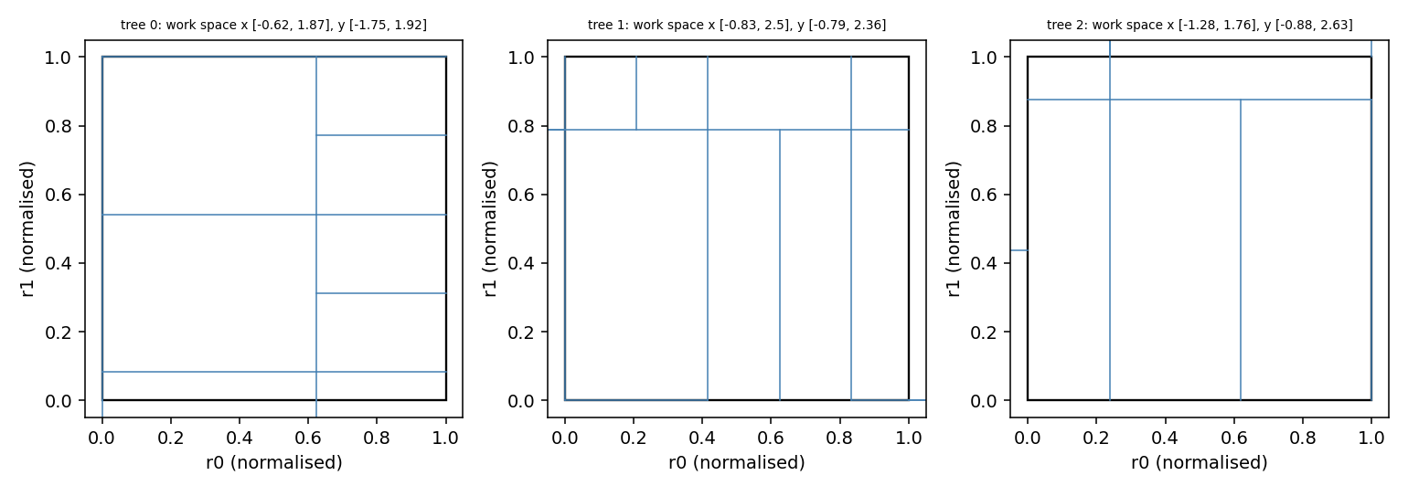
The three trees own the same plane, shown for the first two features, and cut it at different places. The black square is the data domain [0, 1]²; each title gives the work space of the tree.

Two windows of counts. Every node keeps two counters: r, the number of samples of the reference window that reached the node, and l, the number of samples of the latest window. The first window samples fill r. Afterwards every sample is scored with r and counted in l; when window samples have been counted, r takes the value of l and l starts again from zero. The reference always describes the last full window.

The score. A sample follows its path in each tree down to the terminal node: the first node that is at the last level or holds size_limit_frac · window reference samples or fewer (0.1 · window by default). With r* the count of that node and k* its depth, the tree contributes r* · 2^k*, and the sum over the trees is

S = sum over the trees of  r* · 2^k*

A node at depth k that holds a share 1/2^k of the window has r · 2^k = window, so under uniform mass every tree contributes window and S is about n_trees · window. The score reports that against the uniform case:

score = M / (M + S),    M = n_trees · window

It is 1 for a region with no reference sample, 0.5 for uniform mass, and goes to 0 in regions where many healthy samples fall. High means anomalous.

A small case with real numbers: one tree of depth 2 on one feature, cut at 0.5, then at 0.25 and 0.75; window = 4, size_limit_frac = 0.25, reference samples 0.1, 0.1, 0.2, 0.9. The counts are 4 at the root, 3 on the left, 1 on the right.

sample	terminal node	r* · 2^k*	score
0.15	left-left, depth 2, r = 3	3 · 4 = 12	4 / 16 = 0.25
0.9	right, depth 1, r = 1 ≤ 1	1 · 2 = 2	4 / 6 = 0.667
0.4	left-right, depth 2, r = 0	0	4 / 4 = 1.0

3. Smallest example

import numpy as np
from dense_armor.utility.anomaly.hst import HalfSpaceTrees

rng = np.random.default_rng(0)
det = HalfSpaceTrees(n_trees=15, depth=8, window=100, range_init=10, seed=0)

for _ in range(200):
    det.learn_one({
        "a": float(rng.normal(0.0, 0.05)),
        "b": float(rng.normal(0.0, 0.05)),
    })

print(f"healthy  {det.score_one({'a': 0.0, 'b': 0.0}):.3f}")
print(f"anomaly  {det.score_one({'a': 10.0, 'b': 10.0}):.3f}")

healthy  0.082
anomaly  0.875

The healthy point sits where the healthy samples sit, in nodes with many reference samples, so its score is close to 0. The far point is outside the range seen in the first ten samples and falls in nodes with few reference samples, so its score is close to 1. The line between the two is 0.5.

4. On a real arm

The residual of joints 0-3 on a SyntheticArm payload fault. The fault (5 kg added at t = 2 s) shifts the residual by tens of N·m; the healthy run stays within ±0.15 N·m. The detector learns only from the healthy part and scores the whole stream.

from pathlib import Path
from dense_armor.utility.anomaly.hst import HalfSpaceTrees
from dense_armor.utility.datasets import SyntheticArm

ds = SyntheticArm(
    Path("test/fixtures/urdf/panda.urdf"),
    period_s=2.0, rate_hz=50.0, n_cycles=2,
    fault_at_s=2.0, fault="payload", payload_mass=5.0,
    noise_std=(1e-3, 5e-3, 5e-2), seed=0,
)

det = HalfSpaceTrees(feature_keys=["r0", "r1", "r2", "r3"], seed=0)

rows = []
for sig, y in ds.stream():
    q, qd, qdd = ds.trajectory(sig.t)
    tau_nom = ds.nominal_torque(q, qd, qdd)
    x = {f"r{j}": float(sig[f"tau_{j}"] - tau_nom[j]) for j in range(4)}
    rows.append((det.score_one(x), y))
    if y == 0:
        det.learn_one(x)

healthy = [s for s, y in rows if y == 0 and s > 0.0]
fault = [s for s, y in rows if y == 1]
print(f"healthy scored {len(healthy)}  max {max(healthy):.3f}")
print(f"fault   scored {len(fault)}  min {min(fault):.3f}")

healthy scored 30  max 0.109
fault   scored 100  min 0.269

Thirty healthy samples are scored (the first 70 fix the ranges and fill the reference) and the highest of them is 0.109. All 100 fault samples are scored and the lowest is 0.269, above every healthy score.

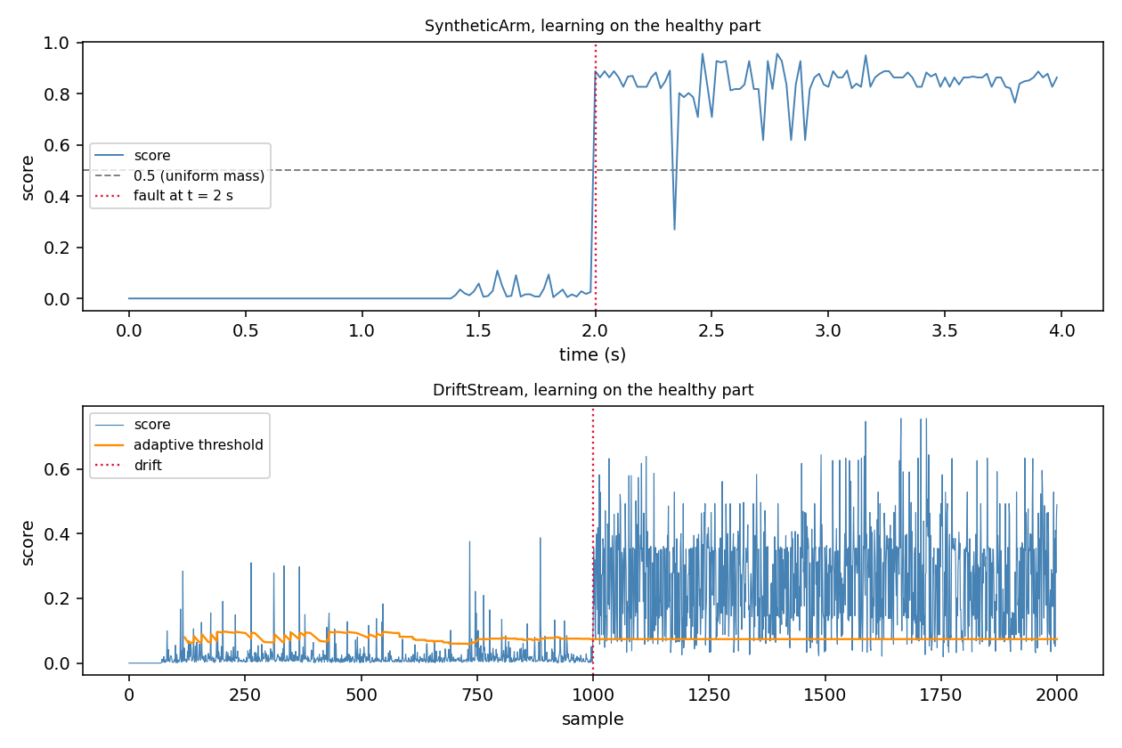
Top: SyntheticArm. The score is 0 for the first samples: the detector needs range_init samples to fix the ranges and window more to fill the reference. Then the healthy samples score close to 0 and the fault jumps above 0.5. Bottom: DriftStream, with the adaptive threshold (the 0.95 quantile of the last 500 scores) in orange.

5. Numbers

SyntheticArm (200 samples, 100 healthy, 100 fault) and DriftStream (2000 samples, one sudden drift at half), the detector at its defaults. The script benchmarks/anomaly_streaming.py regenerates these numbers with two protocols: learn-on-healthy (the detector learns only from the healthy part) and learn-on-all.

Stream	Protocol	ROC-AUC	False alarms on the healthy part	Threshold at the last healthy sample
SyntheticArm	learn-on-healthy	1.000	0.000	1e9
SyntheticArm	learn-on-all	0.863	0.000	1e9
DriftStream	learn-on-healthy	0.982	0.044	0.0741
DriftStream	learn-on-all	0.500	0.044	0.0741

On SyntheticArm the threshold is still 1e9 (flag nothing) at the last healthy sample: the detector scores from sample 70 on and the adaptive threshold needs 50 scores more, and the healthy part has 100 samples; the false-alarm value 0.000 follows from that. With learn-on-all the reference follows the data: after the drift of DriftStream the two windows hold the new regime within 2 · window samples, and the ROC-AUC over the whole stream is 0.500.

The trees and the work spaces are random. Six seeds (0 to 5) give, with learn-on-healthy, ROC-AUC 1.000 on SyntheticArm for every seed and 0.982, 0.985, 0.976, 0.986, 0.983 and 0.969 on DriftStream.

Details

Where the rules come from

The algorithm is Streaming HS-Trees of Tan, Ting and Liu (2011), Fast anomaly detection for streaming data, IJCAI. Page 3: the work space s_q ± 2 · max(s_q, 1 − s_q), Algorithm 1 (a random dimension cut at the mid-point of the current range), Algorithm 2 (the update of the masses r and l), the anomaly score Node*.r × 2^Node*.k summed over the trees, sizeLimit of 0.1 ψ, and the defaults maxDepth = 15, ψ = 250, 25 trees. Page 4: Algorithm 3 (the reference and the latest window, the update every ψ samples). The rule that a split is the mid-point of the node's range is also the one of Ulrich et al. (2025), section 5.2.

Choices stated explicitly

• Window. The paper's window size ψ is window; the default is 50, the paper uses
• The detector scores only after range_init + window samples, and a stream with 100 healthy samples would not reach 250. Measured on the benchmarks with learn-on-healthy: on SyntheticArm window 25, 50 and 70 give ROC-AUC 1.000; on DriftStream window 50, 100 and 250 give 0.982, 0.982 and 0.989.
• Normalisation. The paper assumes features in [0, 1]. The ranges come from feature_ranges or from the first range_init samples (minimum and maximum with a 10 % margin). A value outside the range is not clipped: it falls in the outermost leaves.
• Score scale. M / (M + S) with M = n_trees · window, instead of the raw sum of the paper (high for normal samples). It is 1 for an empty region, 0.5 for uniform mass and 0 for dense regions; the value 0.0 returned before the first reference window is complete is the lowest score. A scale where that placeholder falls in the middle of the healthy scores lowers the ROC-AUC: the 70 samples before the detector is ready look anomalous.
• Size limit. size_limit_frac · window, with size_limit_frac = 0.1, the value the paper suggests.
• Threshold. None means adaptive: the threshold_quantile-quantile (default 0.95) of the last threshold_window scores (default 500); until threshold_warmup scores (default 50) have been seen the effective threshold is 1e9, so nothing is flagged. A float means fixed; 0.5 is the score of uniform mass.

Measured cost

At n_trees=25, depth=15, window=50 with 4 features, on one CPU thread:

• 0.65 ms median and 1.0 ms p99 per learn_one;
• the sample that fixes the ranges builds the trees once and takes 71 to 80 ms;
• memory flat, 52 MB, independent of the stream length (two count tables of n_trees · (2^(depth+1) − 1) integers).

The budget_s declared by the class is 0.1 s: the p99 of a short run includes the one-time construction of the trees.

Limits

The detector counts, it does not model. Two different fault shapes that land in the same region give the same score. The first score comes after range_init + window samples and the first adaptive flag after threshold_warmup more. With learn-on-all a fault that lasts longer than two windows becomes the reference. Other detectors on the same two streams are compared in the overview.

Development diary

The first version of this page described a different detector: a sliding window of exact counts at the leaf, scored -log2((c + 1) / (N + 1)), with one working range for all trees. A review found that its split values were the mid-point of the node's range only when there is one feature (they came from the position of the node in the tree). With learn-on-healthy that version measured ROC-AUC 0.941 on SyntheticArm and 0.907 on DriftStream. Correcting only the split values gave 1.000 and 0.756, and its smallest example did not separate the healthy point from the far one. Replacing the window, the work space and the score with the design of Tan et al. gave the numbers of section 5.