Adam

Adam decides how much a learning model should change its numbers after each example. It remembers how the changes have been going recently and uses that to take steps of a similar size for every number.

Adam is the optimizer that keeps two running averages of the gradient: the first moment, and the second moment. It uses the ratio of the two to build a step that has roughly the same size for every coordinate, on every sample. The step is bounded by the learning rate, and the bias of the two running averages is corrected at the start. This page shows the update, the effect of the learning rate, and the source paper it comes from.

1. What it does

AdaGrad divides the gradient by the square root of its accumulated energy. That energy never decreases, so the step shrinks forever. Adam replaces the accumulator with an exponentially weighted average of the squared gradient, which forgets the distant past and adapts to the recent scale. It also keeps a running average of the gradient itself, which acts as a momentum term.

The update on one sample:

m_t = beta1 * m_{t-1} + (1 - beta1) * g_t
v_t = beta2 * v_{t-1} + (1 - beta2) * g_t^2
m_hat = m_t / (1 - beta1^t)
v_hat = v_t / (1 - beta2^t)
w_{t+1} = w_t - lr * m_hat / (sqrt(v_hat) + eps)

m_t is the running mean of the gradient, v_t is the running mean of its square. beta1, beta2 are the decay rates (default 0.9 and 0.999). The 1 - beta^t correction at the denominator compensates the fact that both averages start from zero: without it, the first few steps would be tiny. lr is the step size, eps a small guard. Suppose w = [0, 0], g = [1, 1], lr = 0.1, and t = 1. Then

m_1 = 0.9 * 0 + 0.1 * [1, 1] = [0.1, 0.1]
v_1 = 0.999 * 0 + 0.001 * [1, 1] = [0.001, 0.001]
m_hat = [1, 1]
v_hat = [1, 1]
w_new = [0, 0] - 0.1 * [1, 1] / (1 + 1e-8)
      = [-0.1, -0.1]

The bias correction is what makes the first step this large. Without it, the step would be 0.1 * 0.1 / sqrt(0.001) = 0.316, which is 3x the final lr.

2. The two forms

The object form owns its state and offers step(weights, gradient) -> weights:

import numpy as np
from dense_armor.utility.optim import Adam

opt = Adam(lr=0.1)
w = opt.step(np.zeros(2), np.array([1.0, 1.0]))
print(w)

[-0.1 -0.1]

The pure form is the pair init_state(dim) and update(state, weights, gradient) -> (state, weights). It works on JAX arrays, so it runs inside jax.jit and jax.lax.scan:

import jax
import jax.numpy as jnp
from dense_armor.utility.optim import Adam

opt = Adam(lr=0.1)
state = opt.init_state(2)
state, w = jax.jit(opt.update)(state, jnp.zeros(2), jnp.array([1.0, 1.0]))
print(w)

[-0.09999935 -0.09999935]

Adam keeps the two running averages and the step counter in the state, so the pure form has more to carry than SGD or AdaGrad. The two forms give the same weights step by step.

3. The learning rate

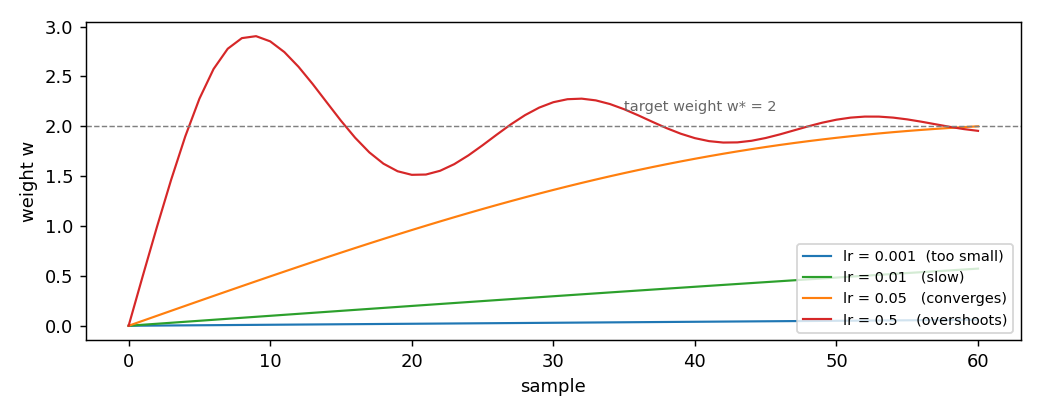
Unlike AdaGrad, Adam's step size does not depend on the scale of the gradient: the ratio m_hat / sqrt(v_hat) has magnitude about 1, so the step is roughly lr regardless of how large the gradient is. This makes the choice of lr the only tuning knob that matters. The figure shows four runs of the same one-feature regression, target weight w* = 2, one per lr:

lr	weight after 1 step	after 10	after 30	after 60
0.001	0.0010	0.0100	0.0300	0.0598
0.01	0.0100	0.0998	0.2960	0.5730
0.05	0.0500	0.4950	1.3621	2.0002
0.5	0.5000	2.8523	2.2419	1.9547

With lr = 0.05 the weight reaches the target around sample 55. With lr = 0.5 the first ten samples overshoot the target, and the weight oscillates around 2 afterwards, because the step size never drops below lr times the normalized gradient. With lr = 0.001 the weight is still at 0.06 after 60 samples: Adam's default lr is conservative, and on short streams it pays.

The lesson: with Adam, lr = 0.05 or larger is worth trying when the default 0.001 is too slow, and lr = 0.5 is already at the edge of the stable region. Unlike AdaGrad, Adam does not shrink its step over time, so lr is a permanent overshoot amplitude and not just a start-up scale.

4. On a real arm

A SyntheticArm from a real Panda URDF gives q, qd, and tau at 50 Hz. The linear model learns the torque of joint 0 as a function of its velocity, one sample at a time. Adam is the optimizer:

from pathlib import Path
import numpy as np
from dense_armor.utility.datasets import SyntheticArm
from dense_armor.utility.linear.glm import LinearRegression
from dense_armor.utility.optim import Adam

ds = SyntheticArm(Path("test/fixtures/urdf/panda.urdf"),
                  period_s=1.0, rate_hz=50.0, n_cycles=8, seed=0)
reg = LinearRegression(optimizer=Adam(lr=0.5, beta1=0.99), intercept=True,
                       feature_keys=["qd0"])
for sig, _ in ds.stream():
    reg.learn_one({"qd0": float(sig["qd_0"])}, float(sig["tau_0"]))
print(round(reg.predict_one({"qd0": 0.5}), 3))

-2.273

Two choices were made to get a sensible value on this stream. First, the learning rate is 0.5 instead of the default 0.001: with 0.001 the weight barely moves after 400 samples. Second, beta1 = 0.99 instead of the default 0.9: the longer memory lets the first moment survive the noise that dominates the short stream. With the default lr = 0.001 the prediction is -0.012, indistinguishable from zero. The value -2.273 is close to the -2.158 of SGD(lr=1e-3) and the -2.824 of AdaGrad(lr=10) on the same stream, so all three converge to the same neighbourhood once Adam's two moments have been given enough time to settle.

The lesson is not that Adam is wrong on short streams. It is that Adam carries two running averages instead of one, and those averages need a few hundred samples to become useful. On a stream of a few hundred samples, a larger lr and a longer beta1 compensate for the short memory.

Details

References

Kingma, D. P., Ba, J. (2014). Adam: A Method for Stochastic Optimization. arXiv:1412.6980, ICLR 2015. Algorithm 1, page 2. Theorem 4.1, page 4, bounds the regret with rate O(sqrt(T)) under bounded gradients ||grad f_t(theta)||_2 <= G, ||grad f_t(theta)||_inf <= G_inf, bounded iterates ||theta_m - theta_n||_2 <= D, ||theta_m - theta_n||_inf <= D_inf, and beta1^2 / sqrt(beta2) < 1, and with the step alpha_t = alpha / sqrt(t) and beta_{1,t} = beta1 * lambda^(t-1), lambda in (0, 1). This implementation uses a constant lr and a constant beta1, so the theorem does not apply to it. Corollary 4.2, page 4, gives the average regret R(T) / T = O(1 / sqrt(T)) under the same schedules.

The update rule in this implementation is Algorithm 1 line by line. The only rename is theta -> w, alpha -> lr, beta -> beta, epsilon -> eps. No simplification, no variant. Adam is the one optimizer in this package where the source and the code coincide exactly.

Choices stated explicitly

• Bias correction kept. The terms 1 - beta1^t and 1 - beta2^t are part of the update. Removing them would make the first steps either tiny (small t, biased m, v) or huge (large t, v under-estimated), as the original paper shows in Section 3 and Figure 4.
• Running averages, not accumulators. v_t is an exponential moving average of g_t^2, not a sum like AdaGrad's G_t. It forgets the past, so on a stationary stream the effective step size does not shrink forever.
• Step size is permanent. The step is lr * m_hat / (sqrt(v_hat) + eps), with no schedule. lr stays relevant at every sample. That is why the stable range of lr in Section 3 is narrower than AdaGrad's.
• eps outside the square root. Algorithm 1 places eps next to sqrt(v_hat), not inside. This matters when v_hat is very small and avoids a division by zero without changing the scale of the square root.

Measured cost

On one CPU thread, a LinearRegression with two features, predict_one plus learn_one per sample, median of 1000 samples after a warm-up of 200: 0.0245 ms per sample, about 76 percent more than SGD and 38 percent more than AdaGrad. The extra work is the two running averages, each updated with a multiply-add per coordinate.

Development diary

The docstring was compared with Algorithm 1 on page 2 of the paper: the five update lines match exactly. The regret theorem needs the decreasing schedules listed in the references, which this implementation does not use. The SyntheticArm example in Section 4 uses lr=0.5 and beta1=0.99 instead of the paper's defaults, because on a 400-sample stream the default lr=0.001 produces a prediction -0.012 that is indistinguishable from zero. The choice is documented in the same section, not hidden.