Streaming anomaly detection
These tools give every new reading a score that says how unusual it is compared with the last few readings, and a yes/no flag when it is too unusual. They answer at once, one reading at a time, without waiting for what comes next.
A robot joint sends its velocity 100 times a second. Most readings are ordinary noise; once in a while one is absurd, because the arm bumped into something or a cable gave a false reading. The controller must know right now, on that very sample, without waiting for the future. The tools on this page give every new sample a score that says how unusual it is compared with the recent past, and a yes/no flag when it is too unusual.
1. Flag a strange sample the moment it arrives
StreamingDeviationDetector takes one value per call and answers True when it deviates.
import numpy as np
from dense_armor.utility.anomaly.streaming import StreamingDeviationDetector

rng = np.random.default_rng(42)
v = 0.5 + 0.1 * rng.standard_normal(3000)
v[1500] = 2.5
det = StreamingDeviationDetector(radius=30, ref_mult=3, n_sigmas=4.0)
flags = np.array([det.update(x) for x in v])
print(np.flatnonzero(flags))
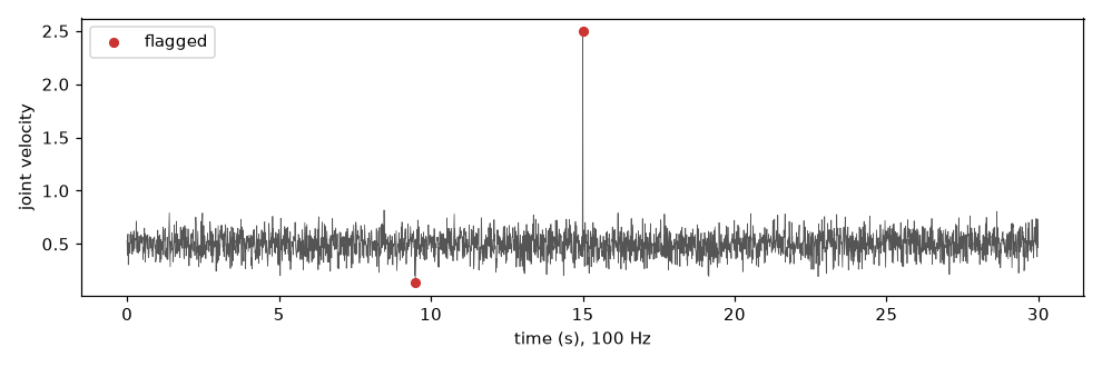
The stream is 30 seconds of a joint velocity around 0.5 with noise 0.1, and one collision at
sample 1500 (value 2.5). The detector flags sample 1500. Sample 4 is the warm-up: with almost
nothing in memory every value looks new, so ignore the first few samples. Sample 949 is one
ordinary noise value that happened to fall far out: one false alarm in 3,000 samples with these
settings. Each call to update looks only at the past, so the answer is available on the same
sample, inside the control loop.
2. How "unusual" is measured
The detector compares the new value with the median of a window of past samples, in units of the window's own spread.
import numpy as np

w = np.array([10, 11, 9, 10, 12, 10, 11, 9, 10])
x = 30.0
med = np.median(w)
mad = np.median(np.abs(w - med))
s = 1.4826 * mad
print(med, mad, round(s, 4), round(abs(x - med) / s, 2))
The score is
$$z = \frac{|x - \mathrm{med}(w)|}{S}, \qquad S = 1.4826 \cdot \mathrm{MAD}(w), \qquad \mathrm{MAD}(w) = \mathrm{med}\big(|w - \mathrm{med}(w)|\big),$$
where:
- $w$ is the window of past samples:
2 * radius * ref_multvalues before the new one; - $\mathrm{med}(w)$ is its median, the "usual" value; unlike the mean, one absurd sample cannot drag it away;
- $\mathrm{MAD}(w)$ is the median distance of the samples from that median, a robust width;
- $1.4826$ turns the MAD into the standard deviation when the noise is normal (it is $1/\Phi^{-1}(3/4)$), so $z$ reads as "how many standard deviations away";
- the sample is flagged when $z$ is larger than
n_sigmas.
In the example the past window is around 10 with MAD 1, so $S = 1.4826$ and the new value 30 is 13.49 standard deviations away: clearly flagged. This robust score is the Hampel identifier (Pearson et al., 2016, "Generalized Hampel filters", EURASIP J. Adv. Signal Process., eqs. 3 and 4).
3. The score itself, as a learn/score estimator
StreamingDeviationScorer gives the number instead of the flag, with the learn_one /
score_one interface used by online-learning pipelines.
from dense_armor.utility.anomaly.deviation import StreamingDeviationScorer

sc = StreamingDeviationScorer(radius=5, ref_mult=2)
for v in [1.0, 1.2, 0.9, 1.1, 1.0, 0.8, 1.05]:
    sc.learn_one({"v": v})
print(round(sc.score_one({"v": 50.0}), 1), round(sc.score_one({"v": 1.1}), 2))
A reading of 50 scores 330.5 standard deviations; a reading of 1.1 scores 0.67, ordinary.
score_one never changes the estimator; learn_one adds the value to the window. A score above
n_sigmas is exactly a flag of StreamingDeviationDetector. It needs the streaming extra:
needs the streaming extra; the install command is on the bridge page of the API reference.
4. The classic robust filters, one sample at a time
dense_armor.utility.anomaly.filters gives the four classic outlier rules as streaming scorers:
Hampel, Tukey fences, Chauvenet and sigma clipping.
from dense_armor.utility.anomaly.filters import HampelScorer

s = HampelScorer(radius=15, n_sigmas=3.0)
for v in [1.0, 1.2, 0.9, 1.1, 1.0, 0.8, 1.05]:
    s.learn_one({"v": v})
print(s.is_outlier({"v": 50.0}), s.is_outlier({"v": 1.1}))
Each scorer looks only at the 2 * radius samples before the value being scored. The batch
versions on the robust filters page use a window centred on the value,
which looks at future samples; a live robot loop cannot, and that is the only difference.
Hampel is shown here; the other three rules are in the Details below.
Precision and recall on 5,000 seeded samples with 50 spikes of size 5–15 (1 % contamination), window 30 (radius 15):
| Scorer | stationary noise (σ = 0.5): precision / recall | sine (amplitude 5, period 500) + same noise: precision / recall | µs per sample |
|---|---|---|---|
| Hampel | 0.459 / 1.000 | 0.318 / 1.000 | 90 |
| Tukey | 0.303 / 1.000 | 0.195 / 1.000 | 75 |
| Chauvenet | 0.282 / 0.980 | 0.167 / 1.000 | 28 |
| SigmaClip | 0.588 / 1.000 | 0.370 / 1.000 | 72 |
Every scorer catches the spikes; precision is the tuning knob. Two things lower it: a trend
inside the window (the sine moves about 1.9 units over 30 samples, and no scorer models a local
slope), and the short window, whose robust scale fluctuates from one window to the next, so a
3-sigma rule fires on some ordinary noise. To raise precision, increase n_sigmas or combine
the scores as pressure_valve does. At 100 Hz (10 ms per cycle) the cost
is under 1 % of the loop budget.
5. All the joints at once
A robot has several joints; MultiChannelStreamingDeviationDetector watches each one with its
own window.
import numpy as np
from dense_armor.utility.anomaly.streaming import MultiChannelStreamingDeviationDetector

rng = np.random.default_rng(0)
qd = 0.1 * rng.standard_normal((500, 6))
qd[300, 2] = 3.0
det = MultiChannelStreamingDeviationDetector(n_channels=6, radius=30, ref_mult=3, n_sigmas=4.0)
flags = np.array([det.update(row) for row in qd])
print(flags[300], np.argwhere(flags[10:]).tolist())
Six joints, one fault on joint 2 at sample 300: row 300 flags only joint 2. After the warm-up
(the first 10 samples are skipped in the print) the list holds [sample − 10, joint]: [290, 2]
is the fault, and [58, 5], [274, 4] are two noise values out of 2,940 checks. Each joint keeps
its own independent window; this is the same rule as step 1, without writing the loop over
joints by hand.
6. Two joints that must agree: online robust Mahalanobis
Some faults are visible only in the combination of channels: each joint alone looks normal,
but together they disagree. OnlineRobustMahalanobis learns how the channels usually move
together and scores how far a sample is from that pattern.
import numpy as np
from dense_armor.utility.anomaly.mahalanobis import OnlineRobustMahalanobis

rng = np.random.default_rng(3)
a = rng.normal(0, 1, 500)
b = a + 0.1 * rng.normal(0, 1, 500)
m = OnlineRobustMahalanobis(feature_keys=["a", "b"])
for x, y in zip(a, b):
    m.learn_one({"a": float(x), "b": float(y)})
print(round(m.score_one({"a": 1.0, "b": 1.0}), 1), round(m.score_one({"a": 1.0, "b": -1.0}), 1))
Two joints that always move together (b follows a). The sample (1, 1) moves them together:
score 1.5, normal. The sample (1, −1) moves them in opposite directions: each value alone is
ordinary (one standard deviation), but the pair is unusual, score 24.7.
The score is the Mahalanobis distance
$$D(x) = \sqrt{\sum_{j=1}^{d} \frac{\langle x - \bar m,\; P_j\rangle^2}{\delta_j}},$$
where $\bar m$ is the robust centre (the geometric median, the point with the smallest total distance to all samples), $P_j$ are the main directions in which the channels vary together and $\delta_j$ how much they vary along each one (eigenvectors and eigenvalues of the median covariation matrix, a robust version of the covariance). Both are updated at every sample by a small step towards the new data:
$$m_{n+1} = m_n + \gamma_{n+1}\,\frac{X_{n+1} - m_n}{\lVert X_{n+1} - m_n\rVert}, \qquad \gamma_n = c_\gamma\,(n + n_0)^{-\gamma},$$
and the same for the covariation matrix with the outer product $(X - m)(X - m)^\top$. Dividing by the distance means one absurd sample moves the estimate by at most $\gamma$, whatever its size: that is what makes it robust. Source: Guillot, Godichon-Baggioni, Robin and Sansonnet (arXiv:2601.03957), the online scheme of section 2.2.
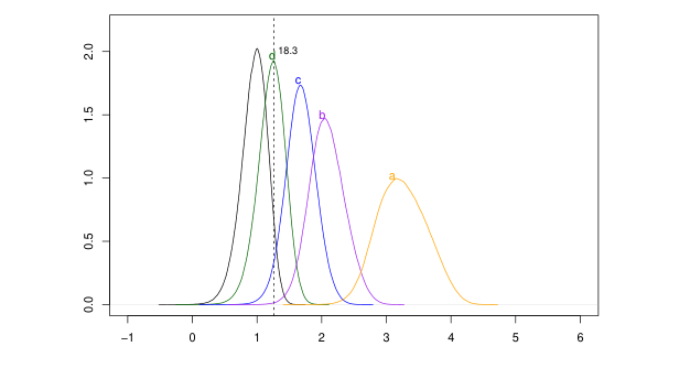
From Guillot et al. (arXiv:2601.03957), Figure 2: density of the (log10) Mahalanobis distance of an outlier under four contamination scenarios (A–D); the dotted line is the inlier threshold. The further a curve sits to the right of the line, the easier the outlier is to flag. Reproduced under the paper's CC BY 4.0 licence.
API reference
streaming 
utility/streaming.py
Promosso da Dense-Evolution-Discovery (Esperimenti 48-49) dopo
validazione su due domini fisici reali indipendenti (braccio robotico
teleoperato SO-101, IMU umano reale UCI HAR) -- stessa disciplina di
promozione gia' usata per stable_frame_filter.py.
MOTIVAZIONE: un robot reale gira a 30-100Hz in tempo reale, non puo'
aspettare un array gia' registrato -- ma leggendo arbiter.classify_
segments riga per riga (non per assunzione) si trova un vincolo reale:
l'etichetta finale spike/regime guarda radius punti AVANTI alla fine
di una sequenza deviante (righe 178-186 di arbiter.py, il controllo
"persiste") per decidere se la sequenza si assesta o torna indietro --
quella meta' non puo' essere streaming a latenza zero. Un vero anello
di sicurezza robotico non ha comunque bisogno di quella distinzione in
tempo reale (e' una domanda di triage, risolvibile dopo); ha bisogno
di "questo punto e' deviante ADESSO" -- esattamente il calcolo per-
punto di classify_segments PRIMA della logica di lunghezza-sequenza.
Solo questa meta' viene portata qui.
CORRETTEZZA: StreamingDeviationDetector, alimentato un punto alla
volta, deve riprodurre esattamente (bit-per-bit) l'array deviante
interno di classify_segments -- verificato su dati reali (non solo
sintetici) in Dense-Evolution-Discovery prima di questa promozione,
ri-verificato qui in test/test_streaming.py sulla telemetria reale
gia' congelata in questo repo (test/agent_v2/telemetry_v2_frozen.jsonl).
PRESTAZIONI: buffer semplice (deque) che ricalcola mediana/MAD ogni passo -- O(span), non una struttura a due heap O(log span). Per le finestre gia' usate in tutto questo progetto (10-100 punti), misurato a ~18.6kHz sostenibile su hardware reale, oltre 180x il tasso reale di un anello di controllo robotico (30-100Hz) -- nessun compromesso di prestazioni reale da giustificare con maggiore complessita'.
SUPPORTO MULTI-CANALE: ogni esperimento robotico reale in Dense-
Evolution-Discovery (le 6 giunture del braccio LeRobot, i piu' assi
dell'IMU) ha richiesto un ciclo manuale per-canale attorno a funzioni
pensate per un solo segnale 1D. classify_segments_multichannel e
MultiChannelStreamingDeviationDetector applicano la STESSA logica
per-canale gia' validata, senza richiedere quel ciclo -- ergonomia, non
un nuovo algoritmo. Ogni canale mantiene la propria finestra di
riferimento e la propria scala indipendenti per costruzione (un giunto
veloce e uno quasi fermo hanno scale di rumore naturali molto diverse;
una scala condivisa desensibilizzerebbe quello lento o darebbe falsi
allarmi su quello attivo).
StreamingDeviationDetector 
StreamingDeviationDetector(
    radius: int = 10,
    ref_mult: int = 3,
    n_sigmas: float = 3.0,
    eps: float = 1e-09,
)
Flag di deviazione causale a latenza zero, un punto alla volta -- stessa finestra causale (radius*ref_mult), stessa mediana/MAD robusta, stessa regola di baseline degenere di classify_segments' (arbiter.py), NON la distinzione spike/regime (che richiede uno sguardo in avanti, resta una domanda batch/offline per design, non una svista).
Examples
det = StreamingDeviationDetector(radius=5, ref_mult=2, n_sigmas=3.0) import numpy as np rng = np.random.default_rng(0) stream = list(rng.normal(0, 1, 20)) + [50.0] # un grande outlier alla fine flags = [det.update(x) for x in stream] flags[-1] True
Source code in dense_armor/utility/anomaly/streaming.py
update 
Alimenta un nuovo punto. Ritorna True se DEVIA rispetto alla
finestra dei punti strettamente PRECEDENTI (mai includendo se
stesso) -- stessa semantica di _window_causal in arbiter.py.
Source code in dense_armor/utility/anomaly/streaming.py
MultiChannelStreamingDeviationDetector 
MultiChannelStreamingDeviationDetector(
    n_channels: int,
    radius: int = 10,
    ref_mult: int = 3,
    n_sigmas: float = 3.0,
    eps: float = 1e-09,
)
N istanze indipendenti di StreamingDeviationDetector, una per
canale -- il flag di ogni canale e' calcolato esattamente come se
StreamingDeviationDetector girasse su quel canale da solo (i
canali non si influenzano mai a vicenda).
Source code in dense_armor/utility/anomaly/streaming.py
update 
x_vec: lunghezza n_channels. Ritorna array bool (n_channels,).
Source code in dense_armor/utility/anomaly/streaming.py
classify_segments_multichannel 
classify_segments_multichannel(
    X: ndarray,
    radius: int = 10,
    ref_mult: int = 3,
    n_sigmas: float = 3.0,
    spike_run_max: int = 2,
    eps: float = 1e-09,
) -> Tuple[np.ndarray, np.ndarray, np.ndarray]
X: (n_campioni, n_canali). Applica classify_segments (arbiter.py)
indipendentemente a ogni colonna -- stesso identico risultato per
canale che chiamarla singolarmente, solo impilato invece di
richiedere un ciclo manuale al chiamante.
Ritorna (etichette, deviazione, incertezza), ognuno (n_campioni, n_canali).
Source code in dense_armor/utility/anomaly/streaming.py
deviation 
Anomaly detectors compatible with an existing online-learning library, built on Dense-Armor's streaming detectors. Needs the optional dependency: the streaming extra
StreamingDeviationScorer 
StreamingDeviationScorer(
    radius: int = 10,
    ref_mult: int = 3,
    feature: str | None = None,
    eps: float = 1e-09,
)
Bases: AnomalyDetector
StreamingDeviationDetector as an anomaly detector of an existing online-learning library.
score_one returns the robust deviation of a value from the causal window of the values
learned before it: |x - median| / scale (median/MAD, as in arbiter.classify_segments),
or |x - median| when the window is flat. learn_one adds the value to the window. A score
above n_sigmas is exactly the case where StreamingDeviationDetector.update returns True.
Parameters
radius
Half-width unit of the causal window; the window holds radius * ref_mult values.
ref_mult
Window length multiplier.
feature
Key of the feature to watch; None takes the feature with the smallest key, so the
result does not depend on the order of the keys. The check_roc_auc of that library (a
multi-feature fraud dataset, downloaded at test time) is skipped: this scorer watches
one feature.
eps
Below this scale the window is treated as flat.
Examples
from dense_armor.utility.anomaly.deviation import StreamingDeviationScorer model = StreamingDeviationScorer(radius=5, ref_mult=2) for v in [1.0, 1.2, 0.9, 1.1, 1.0, 0.8, 1.05]: ... model.learn_one({"v": v}) model.score_one({"v": 1.0}) < 3.0 True model.score_one({"v": 50.0}) > 3.0 True
Source code in dense_armor/utility/anomaly/deviation.py
filters 
utility/streaming_filters.py
Causal (one sample at a time) versions of the four batch robust filters in
robust_filters.py: Hampel, Tukey fences, Chauvenet, iterative sigma
clipping. The batch filters look at a window centred on each point -- they
see the future -- which a robot's real-time control loop cannot do. Each
scorer here looks only at the 2 * radius samples strictly preceding the
value being scored (the causal window) and scores the new value against the
robust centre/scale of that window, in the method's own scale.
The four scorers share the interface of
river_anomaly.StreamingDeviationScorer (learn_one / score_one, feature
selection, is_outlier), so they plug into the pipelines of an existing online-learning library and
anomaly.ThresholdFilter the same way, but each uses its own method's scale
and threshold rather than the median/MAD robust deviation of
StreamingDeviationDetector alone.
HampelFilter is a transformer: learn_one(x) then transform_one(x)
returns the value, or the causal-window median when the value is an outlier
(the same replacement rule as the batch hampel_filter).
Conventions: see SKILL.md. Causal window = 2 * radius samples strictly
before the value being scored; the value is never part of its own window.
See ISTRUZIONI.md, section "Important: centred vs causal windows".
HampelScorer 
HampelScorer(
    radius: int = 10,
    n_sigmas: float = 3.0,
    feature: str | None = None,
    eps: float = 1e-09,
)
Bases: AnomalyDetector
Hampel outlier scorer on the causal window.
The score is |x - med| / (1.4826 * MAD), where med and MAD
are the median and median absolute deviation of the 2 * radius
samples strictly preceding the value being scored. This is the same
formula as robust_filters.hampel_filter (Hampel 1974; Davies and
Gather 1993), applied to the causal window instead of the centred one.
is_outlier returns True when the score exceeds n_sigmas.
Parameters
radius
Half-width unit; the causal window holds 2 * radius samples.
n_sigmas
Threshold in scaled-MAD units (default 3.0, the robust "3 sigma" rule).
feature
Key of the feature to watch; None takes the feature with the
smallest key, so the result does not depend on the order of the keys.
eps
Below this scale the window is flat, and the score is +inf when
the value actually deviates from the window median (degenerate scale
is the strongest possible evidence), 0.0 when it does not.
Examples
from dense_armor.utility.anomaly.filters import HampelScorer import numpy as np rng = np.random.default_rng(0) s = HampelScorer(radius=5, n_sigmas=3.0) for v in rng.normal(0, 1, 20): ... _ = s.learn_one({"v": float(v)}) s.score_one({"v": 50.0}) > 3.0 True s.is_outlier({"v": 50.0}) True
References
Hampel, F. R. (1974). The influence curve and its role in robust estimation. JASA 69(346), 383-393. Davies, L., Gather, U. (1993). The identification of multiple outliers. JASA 88(423), 782-792.
Source code in dense_armor/utility/anomaly/filters.py
TukeyScorer 
Bases: AnomalyDetector
Tukey-fences outlier scorer on the causal window.
The score is how far the value lies beyond the fences
[Q1 - k * IQR, Q3 + k * IQR] of the 2 * radius samples strictly
preceding it, expressed in IQR units: 0 inside the fences, positive
outside. This is the batch robust_filters.tukey_fences rule
(Tukey 1977) applied to the causal window: is_outlier returns True
exactly when the batch would flag the point, since "beyond the fences"
is score > 0. On a flat window (IQR == 0) the score is +inf when the
value differs from the degenerate fence and 0.0 when it does not,
matching the batch rule for a flat window.
Parameters
radius
Half-width unit; the causal window holds 2 * radius samples.
k
Fence multiplier (default 1.5, the Tukey standard; 3.0 for
"extreme outliers").
feature
Key of the feature to watch; None takes the smallest key.
eps
Below this IQR the window is treated as flat.
Examples
from dense_armor.utility.anomaly.filters import TukeyScorer import numpy as np rng = np.random.default_rng(0) s = TukeyScorer(radius=5) for v in rng.normal(0, 1, 20): ... _ = s.learn_one({"v": float(v)}) s.is_outlier({"v": 50.0}) True
References
Tukey, J. W. (1977). Exploratory Data Analysis. Addison-Wesley.
Source code in dense_armor/utility/anomaly/filters.py
ChauvenetScorer 
ChauvenetScorer(
    radius: int = 10,
    threshold: float = 0.5,
    feature: str | None = None,
    eps: float = 1e-09,
)
Bases: AnomalyDetector
Chauvenet outlier scorer on the causal window.
The score is N * P(|Z| >= z), the expected number of observations
that would lie at least z = |x - mu| / sigma away from the mean if
the 2 * radius samples strictly preceding it were a Gaussian sample
of size N. This is the criterion of Chauvenet (1863), the same as
the batch robust_filters.chauvenet_criterion, applied to the causal
window.
Direction of the test
Unlike the other three scorers, Chauvenet rejects when the score is
small: N * P counts how many points of a Gaussian sample would be
at least this far out, and the criterion says "reject when this count
is below 0.5" -- i.e. is_outlier returns score < threshold with
threshold = 0.5. This is the natural direction of the formula and
is documented here because it is the opposite of the "high score =
anomalous" convention of the other scorers.
mu and sigma are non-robust (mean and std), exactly as in the
original criterion; on a window that already contains other outliers
they are already distorted before the central point is judged. That is
a known limitation of the original criterion and not specific to this
implementation.
Parameters
radius
Half-width unit; the causal window holds 2 * radius samples.
threshold
Rejection threshold on N * P (default 0.5, Chauvenet's value).
feature
Key of the feature to watch; None takes the smallest key.
eps
Below this scale the window is treated as flat.
Examples
from dense_armor.utility.anomaly.filters import ChauvenetScorer import numpy as np rng = np.random.default_rng(0) s = ChauvenetScorer(radius=10) for v in rng.normal(0, 1, 20): ... _ = s.learn_one({"v": float(v)}) s.is_outlier({"v": 50.0}) True
References
Chauvenet, W. (1863). A Manual of Spherical and Practical Astronomy, Vol. II, Appendix on the Method of Least Squares.
Source code in dense_armor/utility/anomaly/filters.py
SigmaClipScorer 
SigmaClipScorer(
    radius: int = 10,
    n_sigmas: float = 3.0,
    max_iters: int = 5,
    feature: str | None = None,
    eps: float = 1e-09,
)
Bases: AnomalyDetector
Iterative sigma-clipping outlier scorer on the causal window.
On the 2 * radius samples strictly preceding the value, the mean and
standard deviation are recomputed after removing points beyond
n_sigmas, until stable or max_iters; the value is then scored by
|x - mu_clean| / sigma_clean. This is the same rule as the batch
robust_filters.sigma_clip (standard in astronomy), applied to the
causal window. is_outlier returns True when the score exceeds
n_sigmas. On a window whose cleaned scale is degenerate, the score
is +inf when the value deviates from the cleaned mean and 0.0
when it does not.
Parameters
radius
Half-width unit; the causal window holds 2 * radius samples.
n_sigmas
Clipping threshold and outlier threshold (default 3.0).
max_iters
Maximum number of clipping iterations (default 5).
feature
Key of the feature to watch; None takes the smallest key.
eps
Below this scale the cleaned window is treated as flat.
Examples
from dense_armor.utility.anomaly.filters import SigmaClipScorer import numpy as np rng = np.random.default_rng(0) s = SigmaClipScorer(radius=10, n_sigmas=3.0) for v in rng.normal(0, 1, 20): ... _ = s.learn_one({"v": float(v)}) s.is_outlier({"v": 50.0}) True
References
Standard in astronomy; see e.g. Akritas, M. G., Bershady, M. A. (1996). Linear regression for astronomical data with measurement errors and intrinsic scatter. ApJ 470, 706.
Source code in dense_armor/utility/anomaly/filters.py
HampelFilter 
HampelFilter(
    radius: int = 10,
    n_sigmas: float = 3.0,
    feature: str | None = None,
    eps: float = 1e-09,
)
Bases: Transformer
Streaming Hampel filter: replaces outliers with the causal-window median.
transform_one returns the value itself when it is not an outlier
(same rule as :class:HampelScorer), else the median of the
2 * radius samples strictly preceding it. This is the causal
equivalent of the batch robust_filters.hampel_filter replacement
rule. Other keys in the input dict are passed through unchanged.
Parameters
radius
Half-width unit; the causal window holds 2 * radius samples.
n_sigmas
Threshold in scaled-MAD units (default 3.0).
feature
Key of the feature to filter; None takes the smallest key.
eps
Below this scale the window is flat.
Examples
from dense_armor.utility.anomaly.filters import HampelFilter import numpy as np rng = np.random.default_rng(0) f = HampelFilter(radius=5) for v in rng.normal(0, 1, 20): ... _ = f.learn_one({"v": float(v)}) out = f.transform_one({"v": 50.0}) abs(out["v"]) < 5.0 True
Source code in dense_armor/utility/anomaly/filters.py
mahalanobis 
Online robust Mahalanobis distance for multichannel anomaly detection.
Anomaly detection with a robust estimate of the data covariance: the location is the geometric median (a robust alternative to the mean), the dispersion is the median covariation matrix (MCM), and the score is the Mahalanobis distance of the sample from the median under the current MCM. Both the median and the MCM are updated online with averaged stochastic gradient.
The geometric median is initialised by the Weiszfeld algorithm
(Guillot et al. 2025, eq. 6). The MCM is initialised by the empirical
average of the centred outer products instead of the Weiszfeld
offline MCM of Section A.2: with n_init of the order of tens of
samples the average is more stable than the Weiszfeld iteration,
which for small samples can converge to a rank-one solution. The
online averaged stochastic gradient immediately refines the estimate
as soon as new samples arrive. This is a choice, not the paper's
offline initialisation. Without an offline initialisation the ASGD
updates, whose gradients are normalised to unit Frobenius norm, start
from the identity matrix and never reach the scale of the data.
Two steps of the full method are not implemented. First, Guillot et
al. (2025, Section 2.3 and eqs. 4-5) reconstruct the eigenvalues of
the true covariance from the eigenvalues of the MCM by a Robbins-Monro
scheme; that step refines the absolute scale of the distance, because
the MCM eigenvalues under-estimate the variance. Second, eq. 1 scales
the squared Mahalanobis distances by chi2_d(0.5) / med(D_1..n) so
that the median of the corrected distances matches the median of the
chi-squared distribution of order d. Neither is applied here: for
flagging anomalies the MCM metric with a calibrated threshold is
already usable, and the scaling constant would only shift the number
at which the calibration is done. The threshold in this module is the
one the user calibrates, not the chi2_d(0.5) one of eq. 1.
Why the guards are needed. The literal Section 3.2 update of Guillot
et al. (page 7) was reimplemented outside the library (no cap, no
eigenvalue floor) and run on the 100 healthy residuals of the
ISSUE_mahalanobis_punteggio_esplode.md scenario (joint 1 of the
SyntheticArm payload fault, period_s=2.0, rate_hz=50.0,
n_cycles=2, payload_mass=5.0, seed 0), initialised as this
class does with n_init=20 and evaluated on the 80 samples that
follow the initialisation:
c_gamma=1.0: the finaltrace(V_bar)is-2.88e-04(the matrix crossed zero). The number of steps with a non-positive eigenvalue and the maximum score depend on the order of scoring and updating inside a step, on the same 80 samples. Scoring each sample before the update, which is how the detector is used on a stream: 19 of the 80 steps and maximum score11.36. Scoring after the update: 20 of the 80 steps and maximum score5.96.c_gamma=variance of the residual(2.57e-03): 0 steps with a non-positive eigenvalue,trace(V_bar)=+1.37e-03, maximum score3.70with either order.
The cause is the scale of the normalised ASGD step against the scale
of the MCM. With c_gamma=1 the step has Frobenius norm ~0.04 while
V itself is of order 2.6e-03; the running average V_bar
therefore crosses the zero matrix and 1 / delta blows up. The
max_step_frac=0.1 cap and the eigenvalue floor
trace(V_bar) / d * 1e-3 are the two guards that keep the score
bounded without changing the algorithm: on the same 80 samples, with
the guards, the maximum score is below the threshold (see
test_mahalanobis_healthy_scores_stay_below_threshold).
Step index. In Guillot et al. (page 7) gamma_n = c_gamma (n + n0)^(-gamma)
with n counted from the first sample, so the first update after
n_init = 100 uses gamma_101 = 0.0395 c_gamma for gamma = 0.7.
Here n also counts from the first sample (n = n_init + k at the
k-th update) and the offset is one larger,
gamma_n = c_gamma (n + n0 + 1)^(-gamma): the first update uses
102^(-0.7) c_gamma = 0.0393 c_gamma. The averaged estimates use the
weight 1 / (n + 1) with the same n, which is the paper's
1 / (n + 2) for the previous step index. The offset of one in
gamma_n is a choice of this implementation.
References
Guillot, A., Godichon-Baggioni, A., Robin, S. (2025). Online robust covariance and outlier detection. arXiv:2601.03957. Section 2.3 (offline reconstruction of the eigenvalues), Section 3.2 (online algorithm and initialisation), Section 3.3 (streaming version), Section 3.4 (outlier detection). Cardot, H., Cenac, P., Zitt, P.-A. (2013). Bernoulli 19(1), 18-43. Cardot, H., Godichon-Baggioni, A. (2017). TEST 26(3), 461-480.
OnlineRobustMahalanobis 
OnlineRobustMahalanobis(
    c_gamma: float = 1.0,
    gamma_exp: float = 0.7,
    n0: int = 0,
    n_init: int = 100,
    max_step_frac: float = 0.1,
    feature_keys: Sequence[str] | None = None,
    eps: float = 1e-09,
    seed: int | None = None,
    threshold: float = 7.0,
)
Bases: AnomalyDetector
Online robust Mahalanobis scorer for multichannel signals.
learn_one(x) accepts a dict of features (one per channel). For
the first n_init samples the location and the dispersion are
accumulated; at step n_init the geometric median and the
median covariation matrix are estimated offline (Weiszfeld for the
median, average of centred outer products for the MCM). From
n_init + 1 on, both are updated by averaged stochastic gradient
(Cardot et al. 2013, Cardot and Godichon-Baggioni 2017).
score_one(x) returns the Mahalanobis distance
D(x) = sqrt( sum_j (1 / delta[j]) * <x - m_bar, P[:, j]>^2 )
where P[:, j] is the j-th eigenvector of V_bar and
delta[j] is the corresponding eigenvalue of the averaged MCM.
0.0 until the offline initialisation is complete.
Parameters:
| Name | Type | Description | Default |
|---|---|---|---|
c_gamma
|
float
|
numerator of the step size
|
1.0
|
gamma_exp
|
float
|
exponent of the step size; must be in |
0.7
|
n0
|
int
|
warm-up offset in the step size. |
0
|
n_init
|
int
|
number of samples accumulated before the offline
initialisation. The paper uses 100 in the simulations
(section 4.1). Must be at least |
100
|
max_step_frac
|
float
|
cap on the ASGD step length, as a fraction
of the current Frobenius norm of |
0.1
|
feature_keys
|
Sequence[str] | None
|
list of dict keys, one per channel. |
None
|
eps
|
float
|
numerical guard for divisions and degenerate eigenvalues.
Additionally, every eigenvalue of |
1e-09
|
seed
|
int | None
|
unused in this minimal version, kept for interface stability with the full version. |
None
|
threshold
|
float
|
distance above which |
7.0
|
Raises:
| Type | Description |
|---|---|
ValueError
|
on a non-positive parameter or a bad
|
Examples:
>>> import numpy as np
>>> from dense_armor.utility.anomaly.mahalanobis import (
...     OnlineRobustMahalanobis,
... )
>>> rng = np.random.default_rng(0)
>>> model = OnlineRobustMahalanobis(
...     feature_keys=["a", "b"], n_init=200
... )
>>> for _ in range(500):
...     x = rng.standard_normal(2)
...     _ = model.learn_one(
...         {"a": float(x[0]), "b": float(x[1])}
...     )
>>> inlier = model.score_one({"a": 0.0, "b": 0.0})
>>> outlier = model.score_one({"a": 10.0, "b": 10.0})
>>> outlier > inlier
True
References
Guillot, A., Godichon-Baggioni, A., Robin, S. (2025). arXiv:2601.03957. Sections 2.3, 3.2, 3.3, 3.4.
Source code in dense_armor/utility/anomaly/mahalanobis.py
learn_one 
Learn one sample.
Parameters:
| Name | Type | Description | Default |
|---|---|---|---|
x
|
dict
|
dict of one feature per channel. |
required |
t
|
float | None
|
unused. |
None
|
Returns:
| Type | Description |
|---|---|
OnlineRobustMahalanobis
|
|
Source code in dense_armor/utility/anomaly/mahalanobis.py
score_one 
Score one sample.
Parameters:
| Name | Type | Description | Default |
|---|---|---|---|
x
|
dict
|
dict of one feature per channel. |
required |
t
|
float | None
|
unused. |
None
|
Returns:
| Type | Description |
|---|---|
float
|
Mahalanobis distance under the current MCM. |
float
|
the offline initialisation is complete or on a non-finite |
float
|
input. |
Source code in dense_armor/utility/anomaly/mahalanobis.py
is_outlier 
Boolean wrapper around :meth:score_one.
Details
- The other three rules.
TukeyScorer: the normal range is $[Q_1 - 1.5\,\mathrm{IQR},\; Q_3 + 1.5\,\mathrm{IQR}]$ with $Q_1, Q_3$ the quartiles of the window and $\mathrm{IQR} = Q_3 - Q_1$ (window[10, 11, 9, 10, 12, 10, 11, 9, 10]: range $[8.5, 12.5]$).ChauvenetScorer: rejects when $N \cdot \mathrm{erfc}(z/\sqrt 2) < 0.5$; itsscore_onereturns $N \cdot P$, so for Chauvenet a low score means anomalous.SigmaClipScorer: repeatedly removes values beyondn_sigmasstandard deviations and scores against what remains.HampelFilteralso replaces an outlier with the window median. - Window size. A short window reacts faster but its median and MAD are noisier, so more
ordinary samples are flagged (step 1 with
radius=5flags dozens of noise samples; withradius=30, n_sigmas=4.0one in 3,000). - Online robust Mahalanobis, differences from the paper. This module is the minimal version of Guillot et al.: it scores with the eigenvalues $\delta_j$ of the median covariation matrix and does not run the Robbins–Monro step that reconstructs the true variances $\lambda_j$, so the scale of the score is larger than the classical chi-squared one (threshold 7.0 by default). It also centres the outer product on the averaged median $\bar m$ and averages with weight $1/n$ (the paper uses $m_n$ and $1/(n+2)$).
- Provenance.
StreamingDeviationDetectoris the causal per-sample half of the Arbiter's per-point deviation check; the spike-versus-regime label needs to see the end of a run and stays batch-only. It was promoted from Dense-Evolution-Discovery after validation on two real physical domains (SO-101 robot arm, UCI HAR inertial data).