Online optimizers

When a model learns, it changes its numbers a little after every example. An optimizer is the rule that decides how big each change is. This page compares the five rules in the library and helps you choose one.

An optimizer is the algorithm that decides how much to change the weights of a linear model on each new sample. It is the only place where the learning rate lives. It is also what separates the five methods in dense_armor.utility.optim. This page starts from the gradient rule. It ends with the choice of optimizer for a stream of robot joint readings.

1. What an optimizer does

A linear model predicts a target with a weighted sum of its inputs. On each sample the model compares the prediction with the target. The comparison gives an error. The optimizer takes that error and turns it into a change of the weights. Same model, same stream, different optimizer: a different fit, and a different reaction when the stream changes.

The simplest rule is gradient descent. The model computes a gradient g of its loss with respect to the weights w. The optimizer moves the weights in the direction opposite to the gradient. It moves them by an amount proportional to a scalar lr, the learning rate:

w_{t+1} = w_t - lr * g_t

w_t are the weights before the update. g_t is the gradient of the loss on the current sample. lr is a positive scalar. Suppose w = [0, 0], g = [2, -4], and lr = 0.5. Then

w_new = [0, 0] - 0.5 * [2, -4] = [-1, 2]

Every optimizer in this package refines this single rule. The refinement decides how far to move on each coordinate. To do that, it uses the history of the gradients seen so far. SGD is the rule above, with no refinement. The other four add a memory.

2. The two forms

Every optimizer is exposed twice. The object form owns its state. It offers step(weights, gradient) -> weights:

import numpy as np
from dense_armor.utility.optim import SGD

opt = SGD(lr=0.1)
w = np.zeros(2)
w = opt.step(w, np.array([1.0, 0.5]))
print(w)

[-0.1  -0.05]

The pure form is a pair: init_state(dim) and update(state, weights, gradient) -> (state, weights). It works on JAX arrays. It takes the state as an argument. It returns a new state instead of writing to the object. So it runs inside jax.jit and jax.lax.scan:

import jax
import jax.numpy as jnp
from dense_armor.utility.optim import SGD

opt = SGD(lr=0.1)
state = opt.init_state(2)
w = jnp.zeros(2)
state, w = jax.jit(opt.update)(state, w, jnp.array([1.0, 0.5]))
print(w)

[-0.1  -0.05]

The two forms share the same hyper-parameters and the same arithmetic. A stream run inside jax.lax.scan gives the same weights as the same stream run one step at a time. The models in dense_armor.utility.linear use the pure form. The tests use the object form.

3. The five optimizers

SGD moves every coordinate by the same amount. The four others adapt the step to the gradient history of each coordinate.

• SGD(lr) follows the raw gradient. It is the reference against which the others are measured. Choose it when the data has no strong per-coordinate scale difference.
• AdaGrad(lr, eps) accumulates the squared gradient per coordinate. It divides the step by the square root of that accumulator. A coordinate with a large past gradient moves less. It is the first choice when some features are rarely informative. This is a variant of Algorithm 4.1 of Orabona (2019): the source uses a per-coordinate step size that depends on the diameter along each coordinate D_i; here a single scalar lr is shared by all coordinates.
• Adam(lr, beta1, beta2, eps) keeps a running mean and a running variance of the gradient. Both are bias-corrected. It behaves like AdaGrad on sparse gradients and like a momentum method on dense ones.
• FTRLProximal(alpha, beta, l1, l2) minimises a regularised version of the accumulated losses. It does not follow the current gradient directly. The L1 term sets to zero every weight whose accumulated evidence has not crossed l1. That makes the weights sparse. The source of the soft threshold is Example 7.24 of Orabona (2019), which uses a time-varying L1 coefficient lambda * t. The FTRL-Proximal of McMahan (2011), page 2, Table 1, also uses a cumulative L1 penalty t * lambda; this implementation keeps l1 constant, which changes the schedule of the L1 penalty.
• OnlineNewtonStep(gamma, eps, D) keeps a running approximation of the Hessian. It uses the inverse of that approximation as a preconditioner. The update follows Figure 3 (page 10 of the manuscript) of Hazan, Agarwal and Kale (2007); Orabona (2019), Algorithm 7.6 (Section 7.10), states the algorithm in argmin form. Hazan et al. give a logarithmic regret on exp-concave losses on a bounded set; OnlineNewtonStep.from_bounds builds the optimizer with their constants and the projection. On a generic squared loss there is no guarantee, and the table below shows a case where the method does not converge.

4. On a real arm

A SyntheticArm from a real Panda URDF gives q, qd, and tau at 50 Hz. The linear model learns the torque of joint 0 as a function of its velocity. It learns one sample at a time. SGD is the optimizer:

from pathlib import Path
import numpy as np
from dense_armor.utility.datasets import SyntheticArm
from dense_armor.utility.linear.glm import LinearRegression
from dense_armor.utility.optim import SGD

ds = SyntheticArm(Path("test/fixtures/urdf/panda.urdf"),
                  period_s=1.0, rate_hz=50.0, n_cycles=2, seed=0)
reg = LinearRegression(optimizer=SGD(lr=1e-3), intercept=True,
                       feature_keys=["qd0"])
for sig, _ in ds.stream():
    reg.learn_one({"qd0": float(sig["qd_0"])}, float(sig["tau_0"]))
print(round(reg.predict_one({"qd0": 0.5}), 3))

-2.158

The stream carries a friction term on joint 0. SGD absorbs part of that term into the single weight. The prediction at a velocity of 0.5 rad/s is the torque the model expects at that velocity. Swap SGD for any of the other four. The same three lines run unchanged. The optimizer is the only moving part.

5. Which one on a stream with a sudden change

The same two-feature regression, 400 samples, one LinearRegression per optimizer. The true weights are [1, -2] on the first 200 samples and [-1, 3] on the last 200. The stream changes suddenly at the midpoint. The table reports the mean absolute error on the first 200 samples, the mean absolute error on the last 100 (the first 100 after the change are excluded as transient), and the median per-sample latency of predict_one plus learn_one on one CPU thread.

learner                             MAE pre   MAE post   median us
--------------------------------------------------------------------
SGD(lr=0.05)                         0.1624     0.0401        13.1
AdaGrad(lr=0.5)                      0.0773     0.9610        17.0
Adam(lr=0.05)                        0.2772     0.5705        24.1
FTRLProximal(l2=0.1)                 0.1479     0.0536        19.4
OnlineNewtonStep                     1.7168     3.9491        23.8

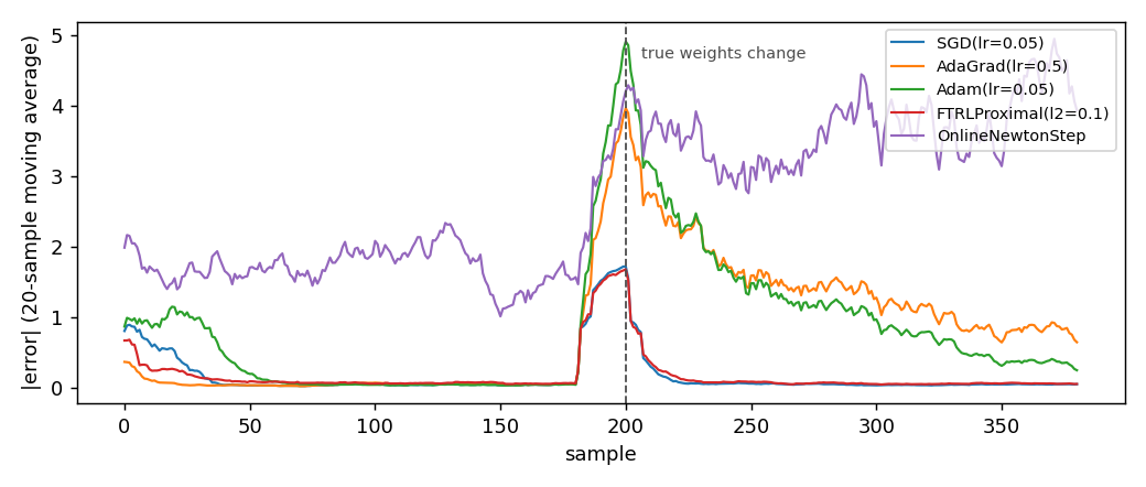
SGD and FTRLProximal follow the change. AdaGrad and Adam are slower to forget the pre-change fit, because their per-coordinate memory was tuned on the old weights. OnlineNewtonStep does not converge on this stream at all. The squared loss is not exp-concave, and the paper gives no guarantee outside that class. The table comes from test/linear/test_comparison_table.py, which prints it at every run.

Details

References

Orabona, F. (2019). A Modern Introduction to Online Learning. SGD is Chapter 2, Algorithm 2.1, with regret Theorem 2.13. AdaGrad is Chapter 4, Algorithm 4.1, pages 45-46, with regret Theorem 4.32; this implementation uses a scalar learning rate in place of the source's per-coordinate D_i, and Theorem 4.32 does not apply to it. FTRLProximal is Chapter 7, Algorithm 7.2; the soft threshold is the proximal operator of the L1 norm, Section 7.8, Example 7.24. The constant l1 form is from McMahan, H. B. (2011), Follow-the-Regularized-Leader and Mirror Descent, AISTATS, Section 3.1. OnlineNewtonStep is Figure 3 (page 10 of the 2008 manuscript) of Hazan, E., Agarwal, A., Kale, S. (2007), Logarithmic regret algorithms for online convex optimization, Machine Learning 69, and Algorithm 7.6 (Section 7.10, page 122) of Orabona (2019). Adam is Kingma, D. P. and Ba, J. (2014), arXiv:1412.6980, Algorithm 1.

Choices stated explicitly

• __eq__ compares only the public hyper-parameters. Two optimizers are equal when their learning rate and decay coefficients match. The internal accumulators (_G, _m, _v, _z, _A_inv) are not part of the identity. Two freshly built optimizers of the same class should compare equal before any sample is seen.
• FTRLProximal ignores the weights argument of update. The FTRL iterate is a function of the accumulated gradient and the step counter alone. The weights from the previous step enter only through the regulariser, which is part of the state. The signature stays uniform for the caller.
• OnlineNewtonStep has no convergence test on the squared loss. The paper's regret bound covers exp-concave losses. On a generic convex loss the method can stall. The table above shows a case where it does.

Measured cost

On one CPU thread, dense_armor.utility.linear.LinearRegression with two features, predict_one plus learn_one per sample, median of 1000 samples after a warm-up of 200:

Optimizer	median per sample
SGD	0.0139 ms
AdaGrad	0.0178 ms
Adam	0.0245 ms
FTRLProximal	0.0194 ms
OnlineNewtonStep	0.0247 ms

The cost of every optimizer is dominated by the model's own arithmetic, the matrix-vector product and the outer product, not by the state update. Pick the optimizer that fits the data. Do not pick by latency unless the loop runs above 10 kHz.

Development diary

The page was written after the optimizers and the linear models were in place. Every number on it was measured against the code that ships. The convergence figure is generated by docs/assets/optim/make_figure.py, which runs the same 400-sample stream as the table.