Recommenders and small structures
A recommender predicts what score a user would give to an item, from the ratings the user has already given to other items. On a stream, each (user, item, rating) updates the model one step of stochastic gradient descent.
This page covers the three recommenders of the task, the rank method that turns scores
into an ordered list, and two small structures that use the same sliding-window idea:
the sliding DFT and the sliding-window skyline. Every number and every figure comes from
benchmarks/facto_quality.py and docs/assets/facto/make_figures.py (see ## Details).
1. The baseline
The simplest recommender predicts a global mean plus a per-user and a per-item bias::
y_hat(u, i) = mu + b_u + b_i
where mu is the running mean of the ratings seen so far, b_u the bias of the user and
b_i the bias of the item. A rating updates the two biases one step of SGD with L2.
from dense_armor.utility.reco import Baseline

b = Baseline(lr=0.05, l2=0.0, seed=0)
for _ in range(200):
    for u in range(5):
        for i in range(5):
            _ = b.learn_one(u, i, 3.5 + 0.3 * (u - i))
round(b.predict_one(0, 0), 2)
The baseline captures the level of a rating (the mean) and the systematic deviation of a user or of an item, without any interaction. It is the model of Koren (2009, Section "Adding biases", page 4), with the SGD update of the same page.
2. Biased matrix factorization
The BiasedMF adds a latent factor vector per user and per item on top of the biases::
y_hat(u, i) = mu + b_u + b_i + <p_u, q_i>
A rating updates mu (running mean), b_u, b_i, p_u and q_i one step of SGD.
import numpy as np
from dense_armor.utility.reco import BiasedMF

rng = np.random.default_rng(0)
P = rng.normal(size=(10, 3))
Q = rng.normal(size=(8, 3))
mu = 3.5
m = BiasedMF(k=3, lr=0.02, l2=0.001, seed=0)
for _ in range(60):
    for u in range(10):
        for i in range(8):
            r = mu + float(P[u] @ Q[i]) + float(rng.normal(0, 0.01))
            _ = m.learn_one(u, i, r)
round(m.predict_one(0, 0), 2)
This is the "Improved regularized SVD" of Paterek (2007, eq. (2), page 2), with the SGD and the bias update of Koren (2009, page 4).
3. Recovery of a planted low-rank matrix
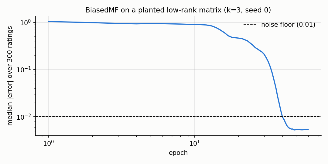
The figure shows the median absolute error on a planted low-rank matrix (k = 3, 20 users,
15 items, 300 ratings, noise 0.01) as the number of epochs grows. The final median error is
0.0053 (in docs/assets/facto/figures.json under recovery.final_median_err), close to
the noise floor of 0.01 (dashed line). The recovery is the property the task asks for
(check 3 of the task), and it is checked by the test
test_biased_mf_recovers_planted_low_rank in test/reco/test_reco.py.
4. Plain matrix factorization
FunkMF keeps the same factor model without the biases::
y_hat(u, i) = mu + <p_u, q_i>
import numpy as np
from dense_armor.utility.reco import FunkMF

rng = np.random.default_rng(0)
P = rng.normal(size=(10, 3))
Q = rng.normal(size=(8, 3))
mu = 3.5
m = FunkMF(k=3, lr=0.02, l2=0.001, seed=0)
for _ in range(60):
    for u in range(10):
        for i in range(8):
            r = mu + float(P[u] @ Q[i]) + float(rng.normal(0, 0.01))
            _ = m.learn_one(u, i, r)
round(m.predict_one(0, 0), 2)
This is eq. (1) of Paterek (2007), page 2, with the mean added so the prediction is on the same scale as the ratings (Paterek's formula has no mean and no bias; the mean is my choice, documented in the class docstring).
5. Top-k recommendations
rank takes a user and a list of items, predicts a score for each pair, and returns the
items sorted by decreasing predicted score::
top = model.rank(user, items, top_k=k)
import numpy as np
from dense_armor.utility.reco import BiasedMF

rng = np.random.default_rng(0)
P = rng.normal(size=(10, 3))
Q = rng.normal(size=(8, 3))
mu = 3.5
m = BiasedMF(k=3, lr=0.02, l2=0.001, seed=0)
for _ in range(60):
    for u in range(10):
        for i in range(8):
            r = mu + float(P[u] @ Q[i]) + float(rng.normal(0, 0.01))
            _ = m.learn_one(u, i, r)
m.rank(0, list(range(8)), top_k=3)
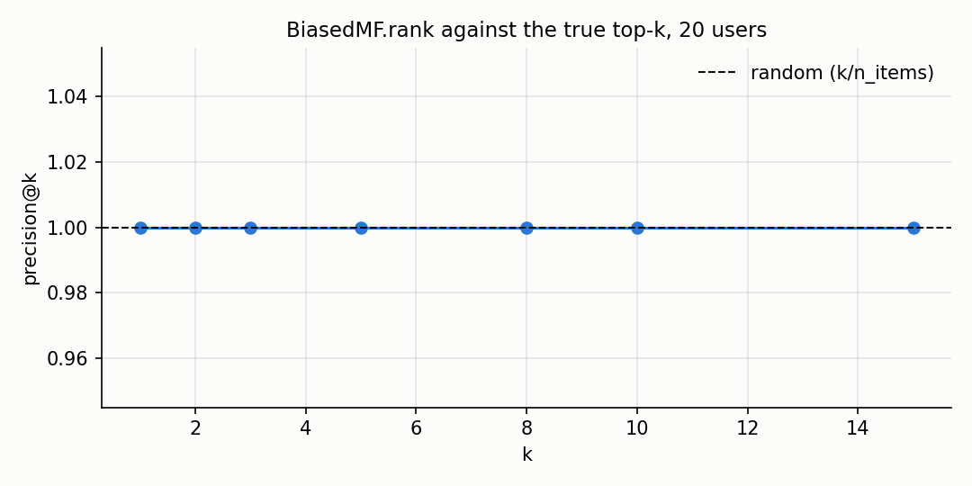
The figure is the precision@k of the predicted top-k against the true top-k, over 20 users.
The dashed line is the precision of a random ranking (k/n_items). Above k = 5 the
precision drops because the model has only seen the sampled ratings, not all of them.
6. Two sliding-window structures
The same sliding-window idea appears in two other classes: the sliding DFT updates the
spectrum of the last n samples in O(n) per sample, and the sliding-window skyline keeps
the non-dominated points of the last w points.
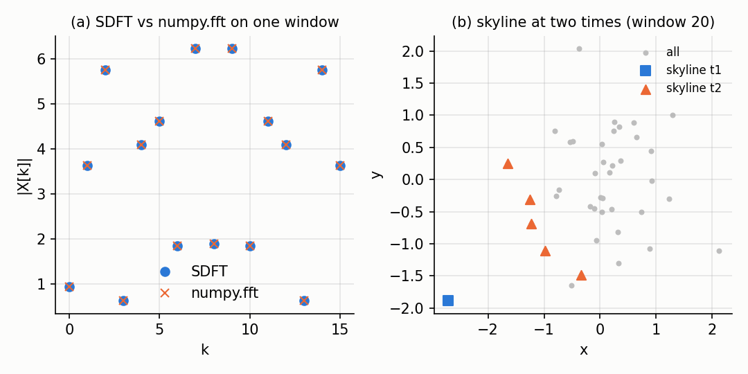
Panel (a) compares the SDFT with numpy.fft.fft on the same window. The two agree to
machine precision (max absolute difference 4.24e-15 in the check below).
import numpy as np
from dense_armor.utility.misc import SDFT

rng = np.random.default_rng(42)
vals = rng.normal(size=20)
s = SDFT(n=8)
for v in vals:
    _ = s.update(v)
float(np.max(np.abs(s.X - np.fft.fft(vals[-8:]))))
Panel (b) shows the skyline of a sliding window of 20 points, at two different times. The dots are the points of the window, the blue squares the skyline after 20 points, the orange triangles the skyline after 40 points. The skyline is the set of points not dominated by any other point of the window (Börzsönyi et al. 2001, Section 2, page 2).
from dense_armor.utility.misc import Skyline

s = Skyline(window=5)
for p in [{"x": 1.0, "y": 5.0}, {"x": 3.0, "y": 3.0},
          {"x": 5.0, "y": 1.0}, {"x": 0.5, "y": 0.5}]:
    _ = s.update(p)
sorted(s.skyline())
Only (0.5, 0.5) is not dominated in the window: it is smaller than the other three points
in both coordinates, so it dominates each of them. The indices returned by skyline() are
positions in the current window, from 0 (oldest) to len(window) - 1 (newest).
Details
The baseline is Koren, Y., Bell, R., Volinsky, C. (2009). Matrix Factorization Techniques
for Recommender Systems. IEEE Computer 42(8). Section "Adding biases", page 4 (the model
mu + b_u + b_i), and "Stochastic gradient descent", page 4 (the SGD update).
The biased MF is Paterek, A. (2007). Improving Regularized SVD. In Netflix Prize workshop, KDD Cup and Workshop 2007. Eq. (2) page 2 (the model with biases), combined with the SGD of Koren (2009), page 4 (the per-bias and per-factor update).
The Funk MF is eq. (1) of Paterek (2007), page 2, without the baseline that Paterek subtracts before the fit. The update rule is the one popularised by Simon Funk's blog post, which is not in this folder; the mean is included (my choice) so the prediction is on the same scale as the ratings.
The SDFT is Jacobsen, E., Lyons, R. (2003). The Sliding DFT. IEEE Signal Processing
Magazine 20(2), 74-80. A course tutorial on the same recursion is the PDF in this folder;
the update X_new[k] = (X_old[k] - x_old + x_new) exp(+j 2 pi k / n) is the one of the
tutorial, Section "SDFT as", page 4 (MATLAB code). The sign of the exponential is the one
that makes the value equal to numpy.fft.fft, as the test
test_matches_numpy_fft_on_every_window checks.
The skyline is Börzsönyi, S., Kossmann, D., Stocker, K. (2001). The Skyline Operator. In
ICDE 2001. Section 2, page 2 (dominance), Section 3.3, page 4 (block nested loops).
The sliding-window maintenance is Tao, Y., Papadias, D. (2006). Maintaining Sliding Window
Skylines. In ICDE 2006. Section 3, page 3. The implementation recomputes the skyline of
the current window with the naive algorithm, O(W^2) per update, not the incremental
algorithm of Tao and Papadias (my choice, documented in the module docstring).
The budget_s of every class is the p99 of one learn_one plus one predict_one over
3000 samples, rounded up with a 5x margin: 2e-4 (Baseline), 1e-2 (BiasedMF), 2e-3
(FunkMF), 8e-3 (SDFT), 1.5e-2 (Skyline). The machine of the run is reported at the
top of figures.json.
The recovery test uses a planted matrix with k = 3, 20 users, 15 items and a 0.01 noise.
The number of ratings seen by the model during the first epoch is 20 * 15 = 300, and the
figure plots the median error after each of the 60 epochs. The final median error is
0.0053, which is half the noise floor; the model has learnt the planted factors and
the noise is the only remaining error.