Payload estimator: sequential recursive least squares for online inertial adaptation

This tool estimates how heavy an object the robot is carrying while the arm is moving, without needing any special weighing tests beforehand. It looks at the real-time forces on the joints, compares them to what an empty robot should feel, and uses a recursive least-squares filter that forgets old samples to update the mass, so it can follow a change when the object is dropped or replaced.

PayloadEstimator estimates the mass of a payload attached to a link of the robot, while the robot is moving. It does not use a pre-recorded identification experiment. It reads the joint torques from the live stream, computes the residual against the unloaded model, and fits a single scalar, the mass, with a recursive least-squares update that forgets old samples. This page shows the update, the fit on a stream where the payload appears at a known time, and the non-negativity constraint on the estimate.

1. What it does

A rigid-body model predicts the torque of each joint from the joint positions, velocities, and accelerations, assuming the model is unloaded. If a payload is attached to a link, the real torques are larger than the prediction by the amount the payload weighs on each joint. The PayloadEstimator uses that residual as a measurement of the unknown mass.

The residual on joint i on a sample:

r_i = tau_i - (M(q) qdd + bias(q, qd) + gravity(q))_i

The gravity torque of a point mass m at link L projected on joint i is m * g * Jz(q)_i, where Jz(q)_i is the vertical component of the Jacobian of the link position with respect to joint i. So the model assumes:

r_i ~ m * phi_i,  with phi_i = g * Jz(q)_i

The unknown is a single scalar m. The estimator updates it with the standard recursive least squares with forgetting. At every sample P is divided by lam once, then the nine joints update m one after the other:

P = P / lam
K = P * phi / (1 + phi * P * phi)
m = m + K * (r - phi * m)
P = P - K * phi * P

P is the scalar covariance of the estimate. lam is the forgetting factor, in (0, 1]. lam = 1 treats all past samples with the same weight; lam < 1 discounts older samples, so the estimate follows a payload that changes over time. The forgetting is applied once per sample, so lam = 0.99 means a memory of about 100 samples (2 s at 50 Hz); the nine joints of a sample then contribute nine scalar updates to the same m. The first sample is skipped, because there is no previous qd to compute qdd.

predict_one() returns max(m, 0), so the estimate is never negative.

2. The two forms

The estimator is used through the standard streaming interface. It takes the Signal from the robot, which carries the joint channels q_j, qd_j, tau_j:

from pathlib import Path
from dense_armor.dynamics.urdf_dynamics import RigidBodyModel
from dense_armor.utility.datasets import SyntheticArm
from dense_armor.utility.linear.payload import PayloadEstimator

model = RigidBodyModel(Path("test/fixtures/urdf/panda.urdf"))
est = PayloadEstimator(model, link="panda_link7", lam=0.99)

ds = SyntheticArm(Path("test/fixtures/urdf/panda.urdf"),
                  period_s=4.0, rate_hz=50.0, n_cycles=1,
                  fault_at_s=2.0, fault="payload", payload_mass=5.0,
                  payload_link="panda_link7", seed=0)
for sig, _ in ds.stream():
    est.learn_one(sig)
print(round(est.predict_one(), 3))

3.362

The estimator also accepts a dict with the same channels, {"q_0": ..., "qd_0": ..., "tau_0": ..., ..., "q_8": ..., "qd_8": ..., "tau_8": ..., "t": ...}, so it can be used on a recorded dataset without wrapping it in a Signal.

The estimate is one scalar. The state is (m, P): the current mass and the current covariance. There is no weight vector, no per-joint adaptation.

3. The forgetting factor

The forgetting factor lam controls how fast the estimate reacts to a change. Values close to 1 treat the whole history equally: on a stationary payload the estimate is stable, but it takes longer to react when the payload changes. Values closer to 0 weight recent samples more: the estimate follows a change quickly but is noisier.

The figure shows three values of lam on the same stream, with a payload of 5.0 kg appearing at t = 2.0 s:

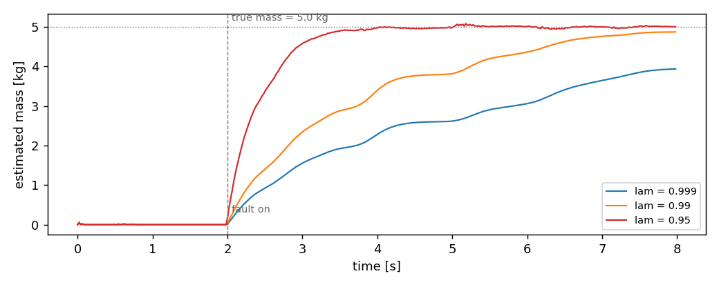
With lam = 0.99 the estimate is 2.88 kg at t = 3.5 and enters the band of 10 % around 5.0 kg 4.26 s after the fault (it is 4.87 kg at the end of the 8 s stream). With lam = 0.95 (a memory of about 20 samples) it enters the band 0.96 s after the fault and ends at 5.00 kg; with lam = 0.999 it has not entered it at the end (3.94 kg). Before the fault the largest value is 0.054 kg, and at t = 1.5 it is 0.0000 kg, which is the correct estimate on an unloaded arm.

The forgetting is what makes the estimator adapt to a payload that appears, disappears, or changes. Without it, lam = 1, the estimate would be the average of everything seen since the start of the stream, and it would take much longer to converge.

4. On a real arm

A SyntheticArm from a real Panda URDF gives q, qd, and tau at 50 Hz. The payload appears at t = 2.0 s as a fault injected by the dataset, with mass 5.0 kg on panda_link7. The estimator follows:

from pathlib import Path
import numpy as np
from dense_armor.dynamics.urdf_dynamics import RigidBodyModel
from dense_armor.utility.datasets import SyntheticArm
from dense_armor.utility.linear.payload import PayloadEstimator

URDF = Path("test/fixtures/urdf/panda.urdf")
model = RigidBodyModel(URDF)

ds = SyntheticArm(URDF, period_s=4.0, rate_hz=50.0, n_cycles=2,
                  fault_at_s=2.0, fault="payload", payload_mass=5.0,
                  payload_link="panda_link7", seed=0)
est = PayloadEstimator(model, link="panda_link7", lam=0.99)
ts, ms = [], []
for sig, _ in ds.stream():
    est.learn_one(sig)
    ts.append(float(getattr(sig, "t", 0.0)))
    ms.append(float(est.predict_one()))

The trajectory of ms over ts:

t	estimated mass
0.50	+0.0000 kg
1.50	+0.0000 kg
2.50	+1.4057 kg
3.50	+2.8762 kg
5.00	+3.8170 kg
7.00	+4.7582 kg

The full trajectory over the 400 samples of the stream has min = +0.0000 and max = +4.8713, and it is never negative. The estimate enters the band of 10 % around the true mass 5.0 kg 4.26 s after the fault and stays there.

Two properties are important here. First, the estimator is online: it does not need a pre-recorded identification experiment, and it follows the change on the same stream that the controller uses. Second, the estimator is bounded below by zero: even if the residual is negative (which can happen because of noise or a small model mismatch), the returned mass never becomes negative, so the downstream controller is never told the payload has negative mass.

Details

References

The method is the standard recursive least squares with an exponential forgetting factor, on a scalar unknown. This is a classical estimator that appears in every textbook on adaptive filtering and system identification; the version used here has no paper-specific formulation.

The overall idea of estimating the inertial parameters of a link online from the live residual is the subject of Foster, J., McCrory, S., DeBuys, C., Bertrand, S., Griffin, R. (2024). Physically Consistent Online Inertial Adaptation for Humanoid Loco-manipulation. arXiv 2405.07901. The paper's method is an Extended Kalman Filter on ten inertial parameters per link, with a log-Cholesky parameterization that keeps the estimate physically consistent by construction. This implementation is a simplification: one scalar (the mass), one estimator (RLS, not EKF), no covariance matrix on the parameters, no log-Cholesky. On the case the paper considers, a known payload on a known link, the two agree on the answer.

The recursive least-squares update with an exponential forgetting factor is a textbook estimator, present in every introduction to adaptive filtering and system identification. The rank-one Sherman-Morrison update without the forgetting term appears in Orabona, F. (2019). A Modern Introduction to Online Learning, Section 7.11 (Vovk-Azoury-Warmuth forecaster), which uses a ridge-style regularization instead of a decay; the two share the same Sherman-Morrison structure. The source cited here does not cover the forgetting factor itself, which is why the docstring of payload.py describes the estimator as standard rather than as derived from a specific paper.

Choices stated explicitly

• Single scalar unknown. The estimator fits one parameter, the mass of the payload. The first moment of the mass (the position of the center of mass on the link) is assumed to be at the link's origin, which is exact only for a point mass placed there. On a real payload the first moment is non-zero and the fit captures a combination of mass and first moment. The paper's ten-parameter-per-link model does not make this approximation.
• Recursive least squares, not Extended Kalman Filter. The update is m += K (r - phi m) with a rank-one update of the scalar covariance. No Jacobian, no matrix inversion, no parameterized manifold. The cost per sample is O(n_joints).
• Forgetting factor lam. The estimate is a weighted average of the residuals seen so far, with weights decaying as lam^k for k samples in the past. Values close to 1 give a stable but slow estimate; values closer to 0 give a reactive but noisy estimate. The default 0.99 has a memory of about 100 samples: on the stream of section 3 it enters the 10 % band 4.26 s after the fault, while lam = 0.95 takes 0.96 s.
• Non-negative output. predict_one() returns max(m, 0). This is a hard constraint on the output, not on the internal state: the internal m can be negative, and only the returned value is clamped. This keeps the downstream controller from receiving a negative mass during the initial transient, when the residual is dominated by noise.
• Forgetting once per sample, one update per joint. The covariance is divided by lam once per sample; the same scalar m is then updated nine times, once per joint of the Panda, as nine independent measurements of the same quantity. An earlier version divided by lam at every joint update, which made the forgetting lam^9 per sample (0.91 for lam = 0.99, a memory of about 12 samples).
• Skipped samples. The first sample (no previous qd), a sample with dt <= 0, a sample with a NaN in q, qd or tau, and a sample without the nine channels are not used; the last two are counted in n_missing.

Measured cost

Each sample requires one call to the rigid-body dynamics (mass_matrix, bias, gravity, and the link Jacobian) plus nine scalar RLS updates. The dominant cost is the dynamics call, not the RLS. On a CPU thread the full stream of n_cycles=2 (400 samples) takes of the order of a minute with the URDF of the Panda, most of which is spent in the JAX compilation of the dynamics on the first sample and in the per-sample evaluation afterwards.

Development diary

The docstring was verified against the source of learn_one. The update rule of the source is the classical RLS with forgetting, and no specific paper claims it. The connection to Foster et al. (2024) is one of theme, not of formula: the paper solves the same problem with a much more elaborate method, and this implementation is a simplification of the idea. The earlier version of the docstring did not make this distinction, and it cited the paper as if the update rule were derived from it. The page now says so explicitly. The figure was generated from a single run of make_figure_payload.py with n_cycles=1 after an earlier attempt with three forgetting factors on n_cycles=2 took more than ten minutes on the CPU thread.