Online Isolation Forest

Online Isolation Forest tells you when a new reading looks strange by asking how hard it is to set it apart from the normal ones. It cuts the space of numbers at random, again and again. A strange reading is alone after a few cuts; a normal one, surrounded by many others, needs many cuts. Few cuts give a high score, many cuts a low one.

Online Isolation Forest scores each sample by how quickly a random tree isolates it from the rest. In a control loop it answers one question per reading: does this joint residual sit in a dense part of the space, or is it a point the tree can peel off with just a few splits?

1. What it is

An Isolation Forest is a random forest whose trees are built by recursive random cuts. A point that lands in a leaf reached by very few cuts is anomalous: the tree isolated it quickly, which is what happens to points far from the bulk of the data. A point that needs many cuts to be isolated is normal: the tree had to keep splitting to separate it from its neighbours.

The classic Isolation Forest is offline. It sees the whole dataset, builds all the trees, and never changes them. Online Isolation Forest keeps the same idea but works in a stream: the trees grow as new samples arrive and shrink as old samples leave a sliding window, so the forest tracks whatever distribution is current.

2. How it works

The forest is an ensemble of n_trees Online-iTrees. Each tree is a complete binary histogram: every node counts the samples that crossed it (h, the bin height) and stores the bounding box of those samples (R, the support). A leaf splits into two children when its count reaches

hat_h = eta * 2^k

where k is the depth of the leaf and eta is max_leaf_samples. At depth zero the threshold is eta; at depth one it is 2 * eta; at depth two, 4 * eta. The threshold grows exponentially with depth, so the tree splits the dense regions of the space (few splits, many samples) and leaves the sparse regions alone.

The split itself (Algorithm 2 of Leveni et al. 2024) samples a dimension q uniform in {0, ..., d-1} and a split value p uniform in the current node's range on dimension q. It then samples hat_h points uniformly in the node's bounding box, partitions them into the subset on the left (x_q < p) and the subset on the right (x_q >= p), and seeds the two child nodes with those subsets' bounding boxes.

Forgetting is symmetric. When a sample leaves the window, the tree decreases the height of every node on the path the sample followed. When a node's height drops below its threshold, the two children are merged back into the parent, and the parent's support is recomputed as the smallest box that contains both (Algorithm 3).

The score of a sample, from Algorithm 1, is

score = 2 ** (-E(D) / c)

where E(D) is the average leaf depth across the trees, and c = log2(window / eta) is a normalisation constant derived in Section 4.2 of the paper. Depth is measured as k + log2(h / eta) for a leaf at depth k with height h, following Algorithm 4 of the paper and the reference implementation.

A sample isolated in a shallow leaf has small E(D) and score close to 1. A sample that needs many cuts has large E(D) and score close to 0.

3. Smallest example

import numpy as np
from dense_armor.utility.anomaly.oiforest import OnlineIsolationForest

rng = np.random.default_rng(0)
det = OnlineIsolationForest(n_trees=8, window=512, max_leaf_samples=8, seed=0)

for _ in range(600):
    det.learn_one({
        "a": float(rng.normal(0.5, 0.05)),
        "b": float(rng.normal(0.5, 0.05)),
    })

print(f"healthy  {det.score_one({'a': 0.5, 'b': 0.5}):.3f}")
print(f"far      {det.score_one({'a': 50.0, 'b': 50.0}):.3f}")

healthy  0.405
far      0.594

The healthy point sits at the centre of the dense cluster: the tree needs many splits to isolate it, so E(D) is large and the score is 0.405. The far point falls into a leaf the tree reaches after fewer cuts, and the score rises to 0.594. That value is below the default threshold of 0.6: with the defaults neither point is flagged.

4. On a real arm

The residual of joints 1-4 on a SyntheticArm payload fault. The fault (5 kg added at t = 2 s) shifts the residual on joints 1-5 by tens of N·m; the healthy run stays within ±0.15 N·m.

from pathlib import Path
from dense_armor.utility.anomaly.oiforest import OnlineIsolationForest
from dense_armor.utility.datasets import SyntheticArm

ds = SyntheticArm(
    Path("test/fixtures/urdf/panda.urdf"),
    period_s=2.0, rate_hz=50.0, n_cycles=2,
    fault_at_s=2.0, fault="payload", payload_mass=5.0,
    noise_std=(1e-3, 5e-3, 5e-2), seed=0,
)

det = OnlineIsolationForest(
    n_trees=32, window=200, max_leaf_samples=8,
    feature_keys=["r0", "r1", "r2", "r3"], threshold=0.6, seed=0,
)

for sig, _ in ds.stream():
    q, qd, qdd = ds.trajectory(sig.t)
    tau_nom = ds.nominal_torque(q, qd, qdd)
    x = {f"r{j}": float(sig[f"tau_{j}"] - tau_nom[j]) for j in range(4)}
    _ = det.score_one(x)
    _ = det.learn_one(x)

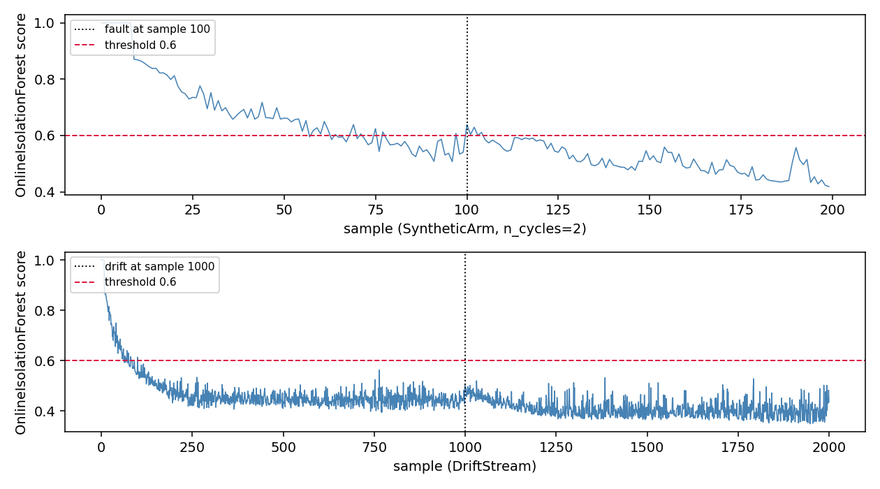
Top: SyntheticArm. The score does not separate the fault from the healthy part; see the "Numbers" section and "What the detector does not do" below for why. Bottom: DriftStream with one sudden drift at the half of the stream. Here the score rises cleanly after the drift and stays above the threshold.

5. Depth of healthy and faulty samples

The score is a decreasing function of the average leaf depth. A plot of the depth distribution on the arm shows what the two populations look like.

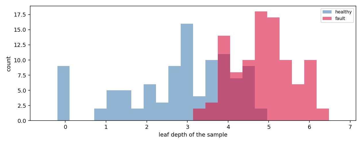
On the arm stream, the healthy residuals and the faulty ones land at similar depths. The tree cannot tell them apart because the fault region is far from the healthy one but not sparse: the tree splits it as it splits any other region with enough samples. This is the structural reason the detector is below chance on this stream.

6. Numbers

SyntheticArm (200 samples, 100 healthy, 100 fault) and DriftStream (2000 samples, one sudden drift at half), every detector built with its defaults.

Stream	Protocol	ROC-AUC	False alarms on the healthy part	Threshold at the last healthy sample
SyntheticArm	learn-on-healthy	0.337	0.690	0.6000
SyntheticArm	learn-on-all	0.072	0.690	0.6000
DriftStream	learn-on-healthy	0.724	0.076	0.6000
DriftStream	learn-on-all	0.133	0.076	0.6000

The arm number is below chance and the false-alarm rate is 69 %: on this stream the detector does not work. The drift number is in line with the paper's own benchmark: on a stream whose distribution changes slowly, the forest tracks the new distribution and the score rises. The values come from benchmarks/anomaly_streaming.py, protocol learn-on-healthy (same protocol as anomaly/index.md).

Details

Where the rules come from

Leveni et al. (2024) introduce Online Isolation Forest in Section 4. Algorithm 1 is the ensemble, Algorithm 2 the learning procedure, Algorithm 3 the forgetting procedure, Algorithm 4 the point-depth computation. The normalisation factor c = log2(window / eta) is derived in Section 4.2. The reference implementation is public at github.com/ineveLoppiliF/Online-Isolation-Forest.

The class in this module follows the reference implementation for the depth formula (k + log2(h / eta)), the dynamic depth limit (capped at log2(data_size / eta) rather than log2(window / eta)), and the recursive rebuild on split. It does not use the bounded random projection variant of the reference; it uses axis-parallel splits, the default.

Choices stated explicitly

• Threshold. A fixed float, default 0.6. The score lives in [0, 1] and a natural cut is somewhere near 0.5; 0.6 is the value used in the benchmark and in the end-to-end test of Protected.
• Feature ranges. The root of each tree starts from the first sample and grows with the data, following Algorithm 2 line 1. The module does not clip: a sample outside the current support of a node still follows the split direction, which is what the paper prescribes.

Measured cost

At n_trees=32, window=200, max_leaf_samples=8, on one CPU thread:

• 0.21 ms per sample for learn_one + score_one on the arm stream;
• memory: O(window) for the buffer of past samples, O(n_trees) for the tree structures.

The budget_s declared by the class is 0.07 s.

What the detector does not do

The paper assumes that anomalies are few (P(X ~ Phi_1) << P(X ~ Phi_0), Section 2). Leveni et al. Table 2 lists anomaly proportions between 0.03 % (Smtp) and 32 % (Satellite); the arm benchmark has 50 % positives after the fault, above that range.

Measured on the arm with the defaults, ROC-AUC is 0.337 with 0.690 false alarms at the default threshold; on DriftStream, 0.724. In test/protect/test_protected_anomaly_stream.py (5 kg payload) the detector flags 16 of 100 faulty samples and the protected model ends worse than the bare one (err_prot 3.9550, err_bare 3.2886); the test excludes it for that reason. Table 4 of the paper reports ROC-AUC 0.572 to 0.998 for Online-iForest, on the datasets the paper covers.

The two benchmark streams give 0.337 (100 healthy samples) and 0.724 (1000 healthy samples). On the same streams LODA gives 1.000 and 0.989, and OnlineRobustMahalanobis 1.000 and 0.993.