Streaming forests: adaptive ensembles and online structural aggregation

A single decision tree relies on a single rule, which breaks the moment a robot's conditions change. A forest combines multiple trees to outvote single-tree errors, using background adaptive detectors to replace failing branches or weighting different tree depths based on their recent prediction accuracy to handle noise and sudden shifts.

1. Why a forest

Picture an AI assistant that must decide, from a few numbers about each incoming request, which of two models should answer it. A decision tree learns that rule one request at a time. The trouble is the day the requests change: the old rule is wrong, and a single tree must notice it, forget, and relearn, with nobody else to lean on.

A forest spreads the risk. Each tree watches its own mistakes. When a tree starts failing it prepares a replacement in the background, and the forest keeps answering with the trees that still work. The two classes below do this in two different ways.

2. Adaptive random forest: replace the trees that go wrong

AdaptiveRandomForestClassifier is the forest of Gomes and colleagues (2017). It has four ideas, each one simple.

Every tree sees every sample, but with a random weight: a sample counts as many times as a Poisson draw with mean 6, so no two trees train on the same data. Every tree also looks at only a few randomly chosen features when it considers a split, which makes the trees differ from one another. Every tree has two small detectors fed with its own mistakes: a warning detector, which is easy to trigger, and a drift detector, which needs more evidence. A warning starts a second tree in the background that trains on the stream but does not vote. If the drift detector then fires, the background tree takes the place of the old one. Finally the forest votes, and each tree's vote is weighted by its recent accuracy.

import numpy as np
from dense_armor.utility.forest import AdaptiveRandomForestClassifier

rng = np.random.default_rng(0)
f = AdaptiveRandomForestClassifier(n_models=5, seed=1)
for i in range(1500):
    x = float(rng.normal(0.0 if rng.random() < 0.5 else 5.0, 0.4))
    y = int(x > 2.5) if i < 750 else int(x <= 2.5)
    f.learn_one({"x": x}, y)
print(f.predict_one({"x": 0.1}), f.predict_one({"x": 5.0}))
print(f.n_warnings_, f.n_drifts_)

1 0
8 2

The stream gives class 0 to small x for the first 750 samples and then swaps the two labels. After the swap the forest answers 1 for x = 0.1 and 0 for x = 5.0, so it has followed the change. Along the way the detectors raised 8 warnings and 2 drifts.

Following a sudden change

A longer test makes the effect visible. DriftStream produces four numbers per sample and changes its rule at sample 1000. The figure shows the accuracy over the last 50 samples, as the median of five seeds, for one adaptive Hoeffding tree and for the forest of ten trees.

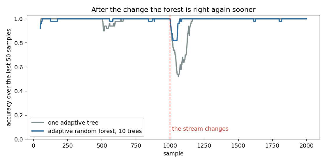
Both fall when the rule changes, and both come back to 1.0. In the median of the five seeds the forest falls less and returns sooner: in the first 100 samples after the change it is right 0.910 of the time and the single tree 0.540. Seed by seed the forest scores 0.90, 0.98, 0.96, 0.91 and 0.84 and the tree 0.12, 1.00, 0.98, 0.53 and 0.54, so the tree is the better one on two seeds and the difference is not significant (Section 4).

The detectors tell the same story from the inside. The next figure counts, for one seed, how many warnings and drifts the ten trees raised.

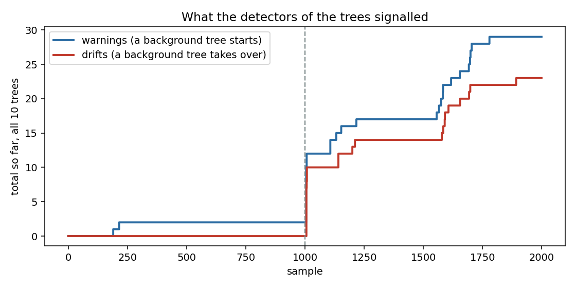
Before the change there are two warnings and no drift: a warning alone replaces nothing. At the change the drift line jumps as the trees are replaced one after another. The forest raised 29 warnings and 23 drifts in total on this stream, and a second burst appears between samples 1550 and 1700, when the rule is no longer changing. With the fast detector setting that is the price of reacting quickly: a tree may be replaced without need. Slower detectors, passed as drift_detector and warning_detector, trade reaction time for fewer false replacements.

The forest costs about 4.3 ms per sample for ten trees against 0.24 ms for the single tree, roughly eighteen times more.

3. Aggregated Mondrian forest: average every depth

A tree has to decide how deep to go. A deep tree follows the data closely but memorises noise; a shallow one is steady but misses detail. AggregatedMondrianForestClassifier and AggregatedMondrianForestRegressor follow Mourtada, Gaiffas and Scornet and skip the decision: the answer is the average of the predictions of every pruning of the tree, each pruning weighted by how well it has predicted up to now. A pruning that has been predicting well counts more; a poor one fades.

There are exponentially many prunings, so the average sounds impossible. The paper shows that with a simple prior, a pruning with n nodes starting at weight 2^-n, the whole sum can be kept as two numbers per node and read along a single path from the leaf to the root. The library implements exactly that, so a prediction costs one walk up the tree.

The library already has a Mondrian forest. It smooths each tree with a fixed prior over where a path leaves the tree, so a node weighs the same whatever it has predicted. The aggregated forest replaces that fixed prior with weights learned from the loss of every node.

from dense_armor.utility.forest import AggregatedMondrianForestRegressor

f = AggregatedMondrianForestRegressor(n_trees=10, seed=0)
for i in range(200):
    x = (i % 20) / 19.0
    f.learn_one({"x": x}, 1.0 if x > 0.5 else -1.0)
print(round(f.predict_one({"x": 0.9}), 2), round(f.predict_one({"x": 0.1}), 2))

0.99 -0.96

The target is -1 on the left half and +1 on the right half; the forest answers 0.99 and -0.96 at x = 0.9 and x = 0.1.

What the weighting does

The next figure uses a noisy curve. The red line is what the leaf alone predicts, which is the prediction of the deepest tree. The blue line is the weighted average of all prunings.

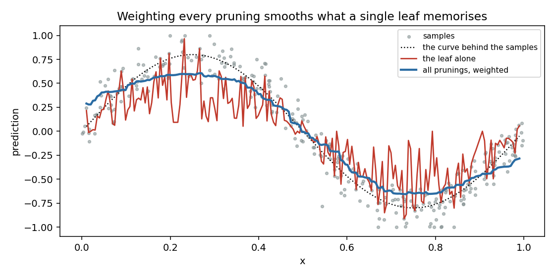
The leaf follows every wiggle of the noise. The aggregated line is smooth and follows the curve, at the cost of flattening the peaks: the average also includes shallow prunings, which predict the middle of a broad region. With a larger step the weights lean harder on the best pruning, and predict_unaggregated_one returns the leaf prediction for comparison.

What the paper guarantees

The paper bounds how much worse the aggregate can be than any single pruning. For the quadratic loss and targets in [-B, B], with step = 1 / (8 B^2), the loss of the forest exceeds that of any pruning T by at most 4 B^2 (|T| + 1) log n; for classification with the logarithmic loss and step = 1, by at most |T| log 2 + (|T| + 1)(K - 1)/4 * log(4n). Against the smallest pruning, the root alone, the bound is just log 2 / step.

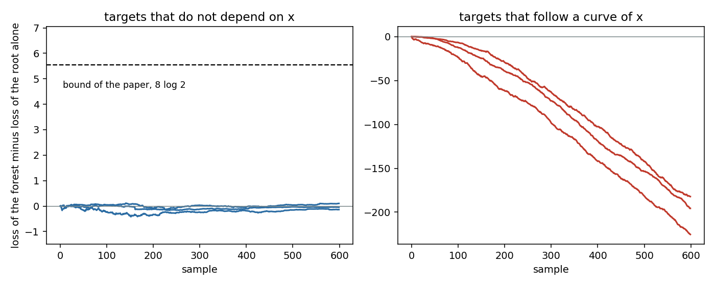
On the left the targets are independent of x, so the root is the best answer, and the forest stays within a fraction of a unit of it, far below the bound of 5.5. On the right the targets follow a curve of x, the aggregate beats the root by more and more, and after 600 samples the difference is between -180 and -225. The bound only limits the damage; it says nothing about how much better the forest can be.

4. Online extra trees: draw the split at random

The random forest and the adaptive random forest ask, for every feature of every leaf, where the best split would be. That is a search: every observed (feature, target) pair is stored, sorted, and scanned. A tree with many leaves, on a stream with many samples, pays for the search at every attempt.

OnlineExtraTreesRegressor (OXT) skips the search. Each leaf draws a small buffer of its first s = 5 observations per candidate feature, takes the minimum and the maximum of that buffer, and picks the split point phi uniformly in that range. From that sample onward, the leaf only keeps two small accumulators, one for the targets below phi and one for the targets above it, and evaluates the variance reduction from those. One candidate per feature, no sorting, no storage of the inputs.

The forest keeps the drift machinery of the adaptive random forest. Every tree sees every sample with probability p = 0.5 (sub-bagging, without replacement). Every tree has two detectors on its own absolute error: a warning, easier to trigger, and a drift, harder. A warning starts a background tree that trains on the same stream but does not vote. If a drift fires, the background tree takes the place of the old one.

import numpy as np
from dense_armor.utility.forest import OnlineExtraTreesRegressor

rng = np.random.default_rng(0)
f = OnlineExtraTreesRegressor(n_models=5, seed=0)
for _ in range(1500):
    a = float(rng.uniform(-1.0, 1.0))
    b = float(rng.uniform(-1.0, 1.0))
    f.learn_one({"a": a, "b": b}, 4.0 * (a > 0.0))
print(round(f.predict_one({"a": 0.5, "b": 0.0}), 1),
      round(f.predict_one({"a": -0.5, "b": 0.0}), 1))

4.0 0.2

The target is 4 when a > 0 and 0 when a < 0; the feature b never matters. After 1500 samples the forest answers close to 4 on the positive side and close to 0 on the negative side, using only random split points and a buffer of five samples per candidate feature.

What the random split costs and buys

The next figure uses the same DriftStream of Section 2, one sudden change at sample 1000, 2000 samples, four features, median of five seeds. The line is the median absolute error, smoothed over 50 samples, for OXT, for MondrianForestRegressor with ten trees, and for AMRulesRegressor.

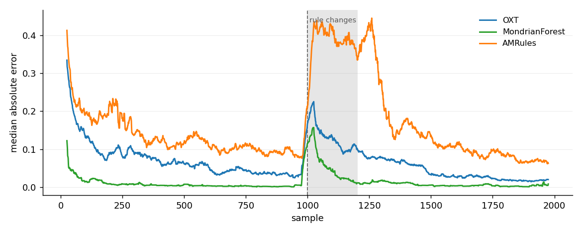
All three fall when the rule changes. OXT recovers more slowly than the Mondrian forest, and its error after the change stays above the Mondrian line. Against AMRules the OXT line stays below the AMRules line both before and after the change.

5. Numbers

DriftStream, one sudden change at half, 2000 samples, four features, median of five seeds, test-then-train. Accuracy (mean squared error of the label for the regressors) on the 300 samples before the change, on the first 100 after it, and on 300 samples starting 200 after it.

learner	before	first 100	after + 200	ms per sample
AdaptiveRandomForestClassifier	0.993	0.910	1.000	4.31
HoeffdingAdaptiveTreeClassifier	1.000	0.540	1.000	0.24
AggregatedMondrianForestClassifier	1.000	0.980	1.000	3.78
MondrianForestClassifier	1.000	0.980	1.000	1.39
AggregatedMondrianForestRegressor (MSE)	0.002	0.084	0.009	3.26
MondrianForestRegressor (MSE)	0.000	0.029	0.001	1.41
OnlineExtraTreesRegressor (MSE)	0.004	0.053	0.007	7.44
AMRulesRegressor (MSE)	0.019	0.213	0.151	0.08

The adaptive random forest has a higher median accuracy than the single adaptive tree in the first 100 samples after the change, but on five seeds the difference is not significant: the forest is better on three seeds and the tree on two (paired Wilcoxon signed-rank, one-sided, p = 0.156; A12 = 0.62, below the 0.71 of a large effect). The forest also has ten trees against one, which is part of the difference. On this stream the aggregated Mondrian forests score the same as or below the Mondrian forests already in the library and cost more per sample; the aggregation also needs a box around the inputs, taken here from the range of the whole stream.

On the same stream OXT scores slightly above the plain Mondrian forest in every window and costs about five times more per sample (7.44 ms against 1.41 ms, twenty trees against ten). Against AMRules the comparison flips: OXT has a lower error after the change (0.053 against 0.213 in the first 100 samples) but is slower (7.44 ms against 0.08 ms). The Mondrian forest has the lower error on all five seeds (A12 = 0.32 for OXT; one-sided paired Wilcoxon with OXT lower, p = 1.000; with five seeds no two-sided p-value can fall below 0.0625). Against AMRules OXT has the lower error on four seeds out of five (p = 0.094, A12 = 0.72), which is not significant at 0.05. The random split is not the winner on this benchmark; its purpose is to remove the split search, and its cost is visible in the millisecond column.

Go or no-go for AMF and OXT

Whether AggregatedMondrianForestRegressor (AMF) and OnlineExtraTreesRegressor (OXT) earn a place next to MondrianForestRegressor was decided on five regimes, 20 seeds each, 1000 samples, mean squared error over the second half of the stream, prequential. The rule, fixed before the run: GO: lower error than the Mondrian forest with two-sided paired Wilcoxon p < 0.05 and the 95% bootstrap interval of A12 above 0.5, or the same error (interval contains 0.5) at no more than half the ms per sample. The script is benchmarks/z_go_nogo.py and the numbers are in benchmarks/z_go_nogo.json (run on Intel(R) Xeon(R) CPU @ 2.20GHz, 4 cores).

regime	model	median error	Mondrian forest	A12 [95% interval]	seeds better	p (two-sided)	ms per sample, model / Mondrian	verdict
20 features, 2 relevant	AMF	0.3584	0.2657	0.04 [0.00, 0.09]	0/20	1.9e-06	2.92 / 3.91	NO-GO
20 features, 2 relevant	OXT	0.1839	0.2657	0.97 [0.94, 1.00]	20/20	1.9e-06	4.15 / 3.91	GO
100 features, 2 relevant	AMF	0.4122	0.3912	0.34 [0.21, 0.46]	4/20	0.0083	2.93 / 16.85	NO-GO
100 features, 2 relevant	OXT	0.3512	0.3912	0.66 [0.50, 0.82]	14/20	0.28	4.72 / 16.85	NO-GO
piecewise function of one feature	AMF	0.0593	0.0313	0.00 [0.00, 0.00]	0/20	1.9e-06	2.86 / 1.32	NO-GO
piecewise function of one feature	OXT	0.0323	0.0313	0.36 [0.23, 0.49]	5/20	0.07	3.92 / 1.32	NO-GO
5% outliers	AMF	1.4647	1.4662	0.45 [0.36, 0.48]	3/20	0.0017	2.81 / 1.32	NO-GO
5% outliers	OXT	1.4526	1.4662	0.52 [0.46, 0.58]	14/20	0.07	3.89 / 1.32	NO-GO
limit of 1 ms per sample (3 trees, 5 for the Mondrian forest)	AMF	0.1139	0.0433	0.00 [0.00, 0.00]	0/20	1.9e-06	0.94 / 0.69	NO-GO
limit of 1 ms per sample (3 trees, 5 for the Mondrian forest)	OXT	0.0802	0.0433	0.00 [0.00, 0.01]	0/20	1.9e-06	1.26 / 0.69	NO-GO

AMF is worse than the Mondrian forest in all five regimes, with a paired p below 0.01 in each; in the regime with 5% outliers the medians differ only in the fourth decimal (1.4647 against 1.4662) and AMF is better on 3 seeds out of 20. OXT is better in one regime only, 20 features with 2 relevant, where it is better on 20 seeds out of 20 (error 0.184 against 0.266) at about the same cost; with 100 features the difference is not significant (p = 0.28), on a piecewise function it ties, and under a 1 ms limit it loses. The decision: keep OXT as an option for streams with many irrelevant features, and do not recommend AMF over the Mondrian forest.

Details

References

• Gomes, H. M., Bifet, A., Read, J., Barddal, J. P., Enembreck, F., Pfahringer, B., Holmes, G., Abdessalem, T. (2017). Adaptive random forests for evolving data stream classification. Machine Learning 106, 1469-1495. Algorithms 1 and 2 (pages 7 and 8 of the PDF), the detector settings on page 17.
• Mourtada, J., Gaiffas, S., Scornet, E. AMF: Aggregated Mondrian forests for online learning. arXiv:1906.10529v2, the manuscript version of the PDF used. Equations 1, 5, 6 and 7, Algorithms 2 and 3, Lemma 1, Corollaries 1 and 2.
• Lakshminarayanan, B., Roy, D. M., Teh, Y. W. (2014). Mondrian forests: efficient online random forests. NIPS.

Choices the papers do not fix

• Detector thresholds. The paper compares a slow setting (delta_w = 1e-4, delta_d = 1e-5) and a fast one (delta_w = 0.01, delta_d = 0.001). The default here is the fast one, which reacts inside streams of a few thousand samples.
• Feature subset. The paper draws the subset when a node is created; here it is drawn at the first split attempt of the node, from the features seen there, and kept for the later attempts. The size is int(sqrt(M)) + 1 unless max_features is given.
• Drift without a warning. The tree is replaced by a new empty tree, since there is no background tree to promote.
• The vote. It adds the class probabilities of each tree, weighted by c / n, and normalises. When every weight is zero the trees count equally.
• Parameter names of the aggregated forest. step is the learning rate eta of the paper and dirichlet is the parameter a of the Dirichlet prior of a node forecaster, (n_y + a) / (n + K a); a = 1/2 is the Krichevsky-Trofimov forecaster. The paper uses neither name.
• Equation 5. The paper prints t - 1 in the denominator of the forecaster. The version that sums to one over the labels of a node uses the count of that node, which is what is implemented.
• Labels and inputs. The set of labels grows with the stream unless classes fixes it. Inputs are clipped to the box [low, high].
• Random predictions. As in the paper, a prediction draws the splits that would separate the query from the sample in its cell and discards them, so predict_one is random and leaves the trees unchanged.

What is implemented

The aggregated forests implement the version of Section 2 of the paper, on an unrestricted Mondrian partition (Algorithm 2). The restricted partition of Section 4, which the paper uses in its experiments and for which it states no guarantee, is not implemented. The regret bounds quoted above are those of the implemented version, for a tree below its max_nodes (default 10000 per tree); once a tree has that many nodes it stops splitting, and the bounds are not claimed for what it predicts after that.

OnlineExtraTreesRegressor and AMRules are left out of the package until their papers are available.

Checks

• The collapsed weights equal the exponentially weighted sum of equation 6 taken over every pruning of a small tree, with a difference below 1e-9 for step from 0.125 to 200 (a leaf of the finished tree stands for all its refinements, which have the same loss, so its prior mass is 1).
• Lemma 1, Corollary 1 and Corollary 2 hold on the prequential streams of test/forest/test_amf.py.
• On a noiseless step function the aggregated prediction with step = 1e4 equals the leaf prediction. On a noisy curve the two differ: with one tree, 300 training samples, queries at 100 of them, and a large step, the two differ by at most 0.19 (median 0.04). A large step selects the best pruning in hindsight, which is the deepest tree only when the data is clean.
• check_estimator passes for the three classes with no check skipped. They have no pure init_state / step form, since the state is a set of trees of changing shape.
• After load_state_dict, a pickle round trip and clone(include_attributes=True), an aggregated classifier still accepts a label it has not seen and returns probabilities that sum to one.

Cost and memory

p99 of one learn_one plus one predict_one over 3000 samples with four features, on a Kaggle CPU: 9.4 ms for the adaptive random forest of ten trees, 4.3 ms for the aggregated classifier and 4.0 ms for the aggregated regressor; budget_s is 0.1 s for the adaptive forest and 0.04 s for the two aggregated forests, about ten times the measured p99.

The trees of both forests are bounded by max_nodes, so the state is constant in the length of the stream. The aggregated trees keep two weights per node and, on uniform inputs with 1, 2 and 4 features, between 3.6 and 4.0 nodes per sample until they reach the limit. The depth of a tree on two features was 21, 30 and 43 after 100, 1000 and 4000 samples.

Development diary

The first test of the collapsed weights against the sum over prunings differed by 0.77. The cause was in the test: the sum of the paper runs over the subtrees of the infinite Mondrian tree, so a leaf of the finished tree has to carry the weight of all its refinements. With that correction the two agree to about 4e-15.

The first test of the adaptive forest expected a drift after a plain label swap. None came: the trees relearn from the weighted samples within about 50 samples, before the drift detector at delta = 0.001 collects enough errors. The warnings came, and the accuracy recovered.