Time series

Robot signals change over time. These tools learn how a signal usually moves, so that they can predict the next value or notice when it behaves differently.

Robot signals are time series. A joint torque repeats with the task cycle, a sensor reading has noise that changes over the day, and the next value of a signal is the natural "normal" to compare the current one against. The four estimators in this section learn one sample at a time and answer one of these questions.

1. The four families

A time-series estimator is a model whose input is the recent past of a signal and whose output is a prediction about the future, a residual, or a smoothed reading. The four families differ in what they predict.

OnlineAR predicts the next value of one channel from its own last order values. A joint torque that follows a periodic pattern is a sequence of AR coefficients, and the model recovers them online. OnlineVAR is the same idea for several channels at once; it predicts every channel from the recent past of every channel, and a group-lasso penalty keeps the coefficients sparse when only a few cross-channel relations matter.

KalmanFilter predicts the state of a system, not its next sample: a position and a velocity, a pose and a bias. The state evolves with a linear model, the measurement says what the sensors saw, and the filter combines the two with the correct weights. Two adaptive variants (VBAdaptiveKalman, InnovationAdaptiveKalman) update the noise covariances from the data themselves when the noise changes.

CycleResidual predicts the value of a repetitive motion at the current phase: it finds the period of the signal, keeps a median template of the last complete cycles, and returns the difference between the current sample and the template (nan until the template exists). When the motion repeats, the residual is small; when something breaks the pattern, the residual jumps.

2. Which one on which stream

stream	what changes	estimator	page
one channel with memory (a torque, a temperature)	the recent past predicts the next value	OnlineAR	ar.md
several channels with cross-dependence (joint positions, sensor bank)	some channels predict others	OnlineVAR	ar.md
a physical state with a model (position, velocity, bias)	the state is hidden, measurements are noisy	KalmanFilter	kalman.md
the same, and the sensor noise itself changes	the noise covariance is not known	VBAdaptiveKalman, InnovationAdaptiveKalman	kalman.md
a repeating motion (a pick-and-place cycle, a rotating joint)	the cycle is the normal	CycleResidual	cycle.md

3. The shared shape

Every estimator in this section learns one sample at a time from a dict, the same way as the rest of the library. OnlineAR with order=1 learns the coefficient of a first-order autoregression from a stream:

import numpy as np
from dense_armor.utility.timeseries import OnlineAR

rng = np.random.default_rng(0)
x = 0.0
ar = OnlineAR(order=1, lam=1.0)
for _ in range(300):
    x = 0.8 * x + 0.3 * rng.normal()
    ar.learn_one({"x": float(x)})
print(round(float(ar.coef_[0]), 4))

0.811

The true coefficient is 0.8, the learned one is 0.81 after 300 samples. With lam = 1.0 the update is ordinary recursive least squares; with a smaller lam older samples weight less, so the coefficient follows a changing signal. The same interface (learn_one, predict_one, transform_one) is shared by every class in the section.

4. On a real arm

A SyntheticArm from a real Panda URDF gives q, qd, and tau at 50 Hz. The arm repeats its motion every second, and a payload of 5 kg appears on the last link at t = 12 s. CycleResidual learns the period and the template of the joint-1 torque in the healthy part, then measures how far every new sample sits from the template:

from pathlib import Path
from dense_armor.utility.datasets import SyntheticArm
from dense_armor.utility.timeseries import CycleResidual

ds = SyntheticArm(
    Path("test/fixtures/urdf/panda.urdf"),
    period_s=1.0, rate_hz=50.0, n_cycles=16,
    fault_at_s=12.0, fault="payload", payload_mass=5.0, seed=0,
)
cr = CycleResidual(period=200, n_cycles=2)
res = []
for sig, _ in ds.stream():
    out = cr.transform_one({"x": float(sig["tau_1"])})
    res.append(out["residual"])

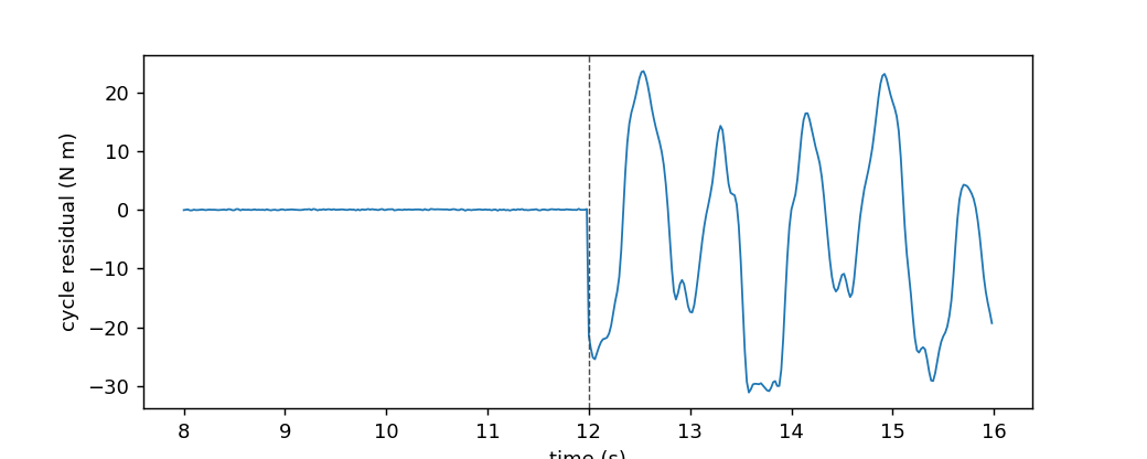
Before the fault the residual is around 0.05 N m; after the fault it is around 12.7 N m, a factor of 266. A control loop that watches this residual sees the change at once, without knowing the payload model.

5. Numbers

The suite runs on a desktop CPU. The default (pytest -m "not slow") is fast: 26 tests in about 5 seconds. The two cycle tests are marked slow because the JAX compilation of SyntheticArm costs about 45 seconds on the first call; with them the full suite is 28 tests in about 50 seconds.

estimator	per-sample	memory class
OnlineAR(order=1)	< 1 ms	O(1)
OnlineVAR(order=1)	< 1 ms	O(1)
KalmanFilter	< 1 ms	O(1)
VBAdaptiveKalman	5 iterations, < 1 ms	O(1)
InnovationAdaptiveKalman	window of 50, < 1 ms	O(window)
CycleResidual(period=200, n_cycles=2)	< 1 ms	O(window)

Details

References

Zaman, B., Lopez Ramos, L. M., Romero, D., Beferull-Lozano, B. (2019). Online topology identification from vector autoregressive time series. arXiv:1904.01864 - the TIRSO algorithm used by OnlineVAR.

Mbalawata, I. S., Sarkka, S., Vihola, M., Haario, H. (2013). Adaptive Metropolis algorithm using variational Bayesian adaptive Kalman filter. arXiv:1308.5875 - the VB-AKF update of VBAdaptiveKalman.

Popescu, M., Mronga, D., Kumar, S., Kirchner, F. (2026). Residual-based adaptive Kalman filtering for legged robot state estimation. arXiv:2608.02316 - the innovation and residual adaptation of InnovationAdaptiveKalman.

Choices stated explicitly

• One sample at a time, dict inputs. Every class in this section follows the same interface as the rest of the library: learn_one(x) takes a dict and returns the estimator, predict_one(x) returns the prediction, transform_one(x) returns the residual or the innovation.
• The four families are independent. OnlineAR/OnlineVAR predict samples, KalmanFilter and its variants predict states, CycleResidual predicts a repeating value. They do not share a base class beyond Transformer.
• The examples use SyntheticArm for the arm, never a hand-written stream. The stream carries the standard joint-state channels at the standard rate.

Measured cost

Per-sample latency is budget_s = 1e-3 s for every class, measured on the author machine as the p99 of learn_one. The cost is dominated by numpy or JAX arithmetic, never by the model state itself. CycleResidual is the only one with a memory_class of O(window): the raw buffer is capped at n_cycles * period + 2 * max_period samples.

Development diary

This section was promoted from the benchmarks/anomaly_streaming.py script that used a cycle residual on the CASPER dataset, the review of the task13-timeseries branch, and the four papers listed above. The first delivery had a delta * I term in OnlineVAR._init and a CycleResidual buffer that grew without bound; both were fixed in the first review round. A second review compared the code with the three papers: OnlineVAR gained the sigma2 ridge of Procedure 2, VBAdaptiveKalman now equals Algorithm 1 at rho = 1, InnovationAdaptiveKalman keeps its constructor arguments and has an adaptive step, and CycleResidual keeps a rolling template.