SGD

SGD is the simplest rule for changing a learning model's numbers after each example: it moves them a little in the direction that reduces the error. The other rules in this section are built on it.

SGD is the simplest online optimizer in the package. It follows the raw gradient, with no memory of the past. Every other optimizer on this page is built on top of it. This page shows the update, the effect of the learning rate, and the regret bound that the source gives.

1. What it does

A linear model computes a gradient g of its loss with respect to the weights w. SGD moves the weights opposite to that gradient, by an amount proportional to a scalar lr, the learning rate:

w_{t+1} = w_t - lr * g_t

w_t are the weights before the update. g_t is the gradient on the current sample. lr is a positive scalar. Suppose w = [0, 0], g = [2, -4], and lr = 0.5. Then

w_new = [0, 0] - 0.5 * [2, -4] = [-1, 2]

That is the whole algorithm. There is no momentum, no adaptive step, no regulariser. SGD is the reference against which the other four methods are measured.

2. The two forms

The object form owns its state and offers step(weights, gradient) -> weights:

import numpy as np
from dense_armor.utility.optim import SGD

opt = SGD(lr=0.1)
w = np.zeros(2)
w = opt.step(w, np.array([1.0, 0.5]))
print(w)

[-0.1  -0.05]

The pure form is the pair init_state(dim) and update(state, weights, gradient) -> (state, weights). It works on JAX arrays, so it runs inside jax.jit and jax.lax.scan:

import jax
import jax.numpy as jnp
from dense_armor.utility.optim import SGD

opt = SGD(lr=0.1)
state = opt.init_state(2)
state, w = jax.jit(opt.update)(state, jnp.zeros(2), jnp.array([1.0, 0.5]))
print(w)

[-0.1  -0.05]

SGD keeps no state: init_state returns an empty dictionary. The two forms give the same weights step by step.

3. The learning rate

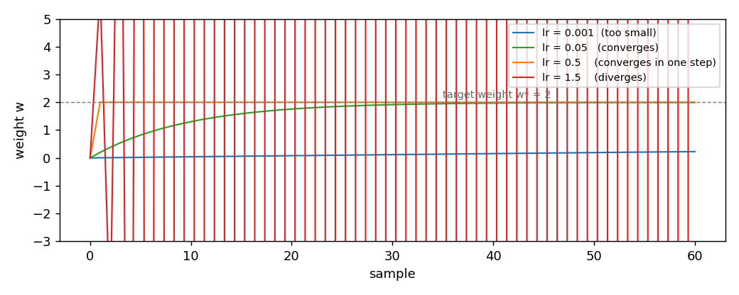
The learning rate is the only hyper-parameter of SGD, and the only choice the caller makes. A small lr learns slowly but never overshoots. A large lr reacts fast and can oscillate or diverge. The figure shows four runs of the same one-feature regression, target weight w* = 2, one per lr:

lr	weight after 1 step	after 10	after 30	after 60
0.001	0.0040	0.0396	0.1166	0.2264
0.05	0.2000	1.3026	1.9152	1.9964
0.5	2.0000	2.0000	2.0000	2.0000
1.5	6.0000	-2046.0000	-2147483646.0000	-2.3e18

With lr = 0.5 the weight jumps to the target in a single step, because for a one-feature quadratic the update w -= lr * 2 * (w - w*) reaches w* exactly when lr = 0.5. With lr = 1.5 the sign of the error flips every step and the magnitude grows without bound. The safe region for lr depends on the curvature of the loss, which the caller usually does not know in advance. A common recipe is to start with a small lr and increase it until the loss stops decreasing.

4. On a real arm

A SyntheticArm from a real Panda URDF gives q, qd, and tau at 50 Hz. The linear model learns the torque of joint 0 as a function of its velocity, one sample at a time. SGD is the optimizer:

from pathlib import Path
import numpy as np
from dense_armor.utility.datasets import SyntheticArm
from dense_armor.utility.linear.glm import LinearRegression
from dense_armor.utility.optim import SGD

ds = SyntheticArm(Path("test/fixtures/urdf/panda.urdf"),
                  period_s=1.0, rate_hz=50.0, n_cycles=2, seed=0)
reg = LinearRegression(optimizer=SGD(lr=1e-3), intercept=True,
                       feature_keys=["qd0"])
for sig, _ in ds.stream():
    reg.learn_one({"qd0": float(sig["qd_0"])}, float(sig["tau_0"]))
print(round(reg.predict_one({"qd0": 0.5}), 3))

-2.158

The stream carries a friction term on joint 0. The single weight absorbs part of it, and the prediction at a velocity of 0.5 rad/s is the torque the model expects at that velocity. A larger lr follows the friction faster but also amplifies the sensor noise. A smaller lr is smoother but lags behind a change of the friction. The trade-off is the same as in the figure above, at the scale of the robot.

Details

References

Orabona, F. (2019). A Modern Introduction to Online Learning. Chapter 2, Algorithm 2.1 (Online Gradient Descent) with a constant step size. Theorem 2.13 gives the regret bound

Regret_T(u) <= D^2 / (2 eta_T) + (1/2) sum_{t=1}^T eta_t ||g_t||^2

for a non-increasing step size eta_t, with D the diameter of the feasible set and g_t the subgradient of the loss on the current sample. The SGD update is the special case V = R^d of the projection step in Algorithm 2.1, so the bound applies with the diameter replaced by the distance between the initial weights and the competitor u.

Choices stated explicitly

• Constant learning rate. The paper's Algorithm 2.1 allows any non-increasing sequence eta_t. SGD takes a single lr at construction and keeps it constant. This is the form the caller asked for and the one that fits the LinearRegression interface.
• No projection. The paper assumes a closed convex feasible set V and a projection step. SGD takes V = R^d, so the projection is the identity and the update is a plain gradient step.
• Numerical guard on lr. The constructor rejects lr <= 0. The paper does not state this, but a non-positive step size would either freeze the weights or reverse the gradient direction.

Measured cost

On one CPU thread, a LinearRegression with two features, predict_one plus learn_one per sample, median of 1000 samples after a warm-up of 200: 0.0139 ms per sample. The cost is dominated by the model's own arithmetic, not by SGD itself.

Development diary

The regret bound was added to this page after the docstring review. The first version of the page quoted only the chapter number, without the theorem; the instruction for the task says the bound must be quoted with its assumptions, so the bound and the diameter assumption are now explicit. The four-rate figure was regenerated for this page; an earlier version used lr = 0.01, 0.1, 1.0, 10.0 and the two middle curves were indistinguishable at the resolution of the plot.