Dependence between channels¶

These tools tell you whether two signals move together, and whether one signal repeats with a regular rhythm, using only the readings seen so far.

What this is¶

A robot has two joints on the same arm. When the operator moves the elbow, the shoulder moves too, because the kinematic chain couples them. A monitoring system wants to know: are these two joints moving together? Is the correlation stable, or has it changed since the payload was attached?

A second question: a joint is oscillating. Is the oscillation random noise, or is there a period — a real vibration at a fixed frequency? Detecting the period means looking at how much the signal agrees with itself at different lags.

This module answers both kinds of questions online, one sample at a time:

Covariance between two channels, and the corresponding Pearson correlation — a number between −1 and 1 that measures how much the two channels move together.
Autocorrelation at lag k — how much a signal agrees with itself k samples in the past. A peak at a specific lag means a period at that lag.

Two flavours of each: running (over the whole history) and rolling (over a bounded window). Running versions react slowly to changes but see everything; rolling versions react quickly and forget deliberately.

Pearson correlation of two channels over a stream that starts
correlated and then decorrelates. The rolling correlation at window=50
follows the change; the running correlation does not.

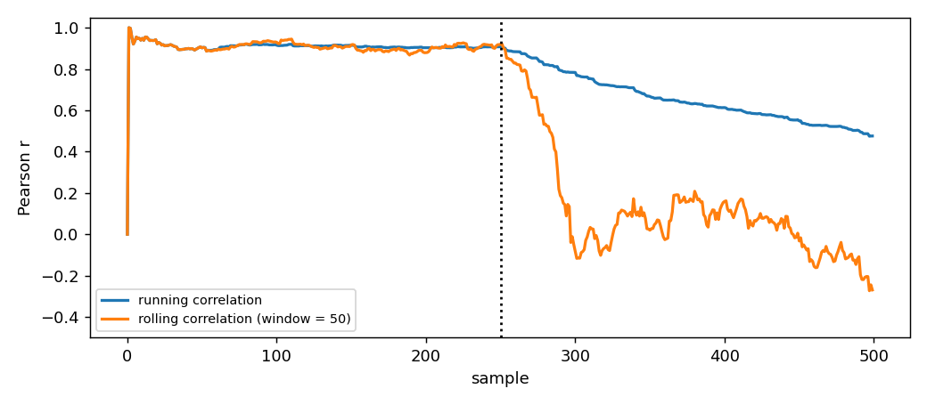
The figure shows two channels that are strongly correlated for the first half of the stream and independent for the second half. The running correlation stays close to the average of the two regimes; the rolling correlation follows the change.

1. The first estimator¶

RunningCovariance keeps the running mean of each channel and the running co-moment, and reads off the covariance and correlation.

from dense_armor.utility.stats.dependence import RunningCovariance

c = RunningCovariance("a", "b")
for a, b in [(1.0, 2.0), (2.0, 4.0), (3.0, 6.0)]:
    c.learn_one({"a": a, "b": b})
print(round(c.cov, 6), round(c.corr, 6))

The output is 2.0 1.0. The stream has b = 2a for all three samples, so the covariance is 2.0 (in the units of a × b) and the correlation is 1.0 (perfectly linearly related).

The class exposes:

c.count — number of sample pairs seen;
c.n_missing — number of pairs skipped because of NaN;
c.cov — sample covariance with n − 1 in the denominator;
c.corr — Pearson correlation coefficient.

The two features to read are named at construction, "a" and "b" in the example. Reading a specific feature requires its name; there is no default for two-channel estimators.

2. Covariance in words¶

The covariance between two streams x₁, …, xₙ and y₁, …, yₙ is

$$ \operatorname{cov}(x, y) = \frac{1}{n - 1} \sum_{i=1}^{n} (x_i - \bar{x})\,(y_i - \bar{y}), $$

where x̄ and ȳ are the sample means.

The formula asks: when x is above its mean, is y above its mean too? If yes for most samples, the products are positive on average and the covariance is positive. If y is usually below its mean when x is above, the products are negative and the covariance is negative. If there is no relation, the positive products cancel the negative ones and the covariance is close to zero.

The scale of the covariance is the product of the units of x and y, so it is hard to interpret directly. The correlation removes the scale:

$$ \operatorname{corr}(x, y) = \frac{\operatorname{cov}(x, y)}{s_x\, s_y}, $$

where s_x and s_y are the sample standard deviations of x and y. The result is always between −1 and 1: +1 for a perfect increasing linear relation, −1 for a perfect decreasing one, 0 for no linear relation.

3. The update: two means and a co-moment¶

Keeping the covariance online is a small extension of Welford's one-channel update. Instead of a single running mean, keep two:

$$ \bar{x}n = \bar{x}{n-1} + \frac{x_n - \bar{x}{n-1}}{n}, \qquad \bar{y}n = \bar{y}{n-1} + \frac{y_n - \bar{y}{n-1}}{n}. $$

Also keep three accumulators:

$$ \begin{aligned} M2_x &\leftarrow M2_x + (x_n - \bar{x}_{n-1})\,(x_n - \bar{x}n), \ M2_y &\leftarrow M2_y + (y_n - \bar{y}{n-1})\,(yn - \bar{y}_n), \ C &\leftarrow C + (xn - \bar{x}_{n-1})\,(y_n - \bar{y}_n). \end{aligned} $$

Here x̄_{n−1} is the mean before the update and x̄_n is the mean after. The three quantities M2_x, M2_y and C are the centered second moments of each channel and the co-moment between them. From those:

$$ \operatorname{cov}(x, y) = \frac{C}{n - 1}, \qquad \operatorname{corr}(x, y) = \frac{C}{\sqrt{M2_x\, M2_y}}. $$

Every symbol is a number kept in memory: two running means, three accumulators, one counter. The update uses only additions, subtractions, multiplications and one division. No sum of squares is ever formed, so the same cancellation that ruins the naive formula for the variance does not occur here.

4. A hand case¶

Take two pairs from the same perfectly linear stream:

(x, y) = (1, 2), (2, 4), (3, 6).

After all three samples:

$$ \bar{x} = 2,\quad \bar{y} = 4,\quad M2_x = 2,\quad M2_y = 8,\quad C = 4. $$

From those:

$$ \operatorname{cov} = C / (n - 1) = 4 / 2 = 2, $$ $$ \operatorname{corr} = C / \sqrt{M2_x \cdot M2_y} = 4 / \sqrt{2 \cdot 8} = 4 / 4 = 1. $$

The code produces exactly these numbers:

from dense_armor.utility.stats.dependence import RunningCovariance

c = RunningCovariance("a", "b")
for a, b in [(1.0, 2.0), (2.0, 4.0), (3.0, 6.0)]:
    c.learn_one({"a": a, "b": b})
print(round(c.cov, 6), round(c.corr, 6))

The output is 2.0 1.0.

5. Merging two partial states¶

Two RunningCovariance states built on disjoint halves of a stream merge exactly, using the pairwise formulas of Chan, Golub and LeVeque (1979):

$$ \begin{aligned} \delta_x &= \bar{x}_B - \bar{x}_A, \ \delta_y &= \bar{y}B - \bar{y}A, \ \bar{x} &= \bar{x}A + \frac{n_B}{n_A + n_B}\,\delta_x, \ \bar{y} &= \bar{y}A + \frac{n_B}{n_A + n_B}\,\delta_y, \ M2_x &= M2{x,A} + M2{x,B} + \frac{n_A\, n_B}{n_A + n_B}\,\delta_x^2, \ M2_y &= M2{y,A} + M2{y,B} + \frac{n_A\, n_B}{n_A + n_B}\,\delta_y^2, \ C &= C_A + C_B + \frac{n_A\, n_B}{n_A + n_B}\,\delta_x\,\delta_y. \end{aligned} $$

The result is exactly what a single accumulator would have produced from both halves together.

from dense_armor.utility.stats.dependence import RunningCovariance

c = RunningCovariance("a", "b")
for a, b in [(1.0, 2.0), (2.0, 4.0), (3.0, 6.0)]:
    c.learn_one({"a": a, "b": b})
print(round(c.cov, 6), round(c.corr, 6))
a = RunningCovariance("a", "b")
b = RunningCovariance("a", "b")
for x, y in [(1.0, 1.0), (2.0, 2.0), (3.0, 3.0)]:
    a.learn_one({"a": x, "b": y})
for x, y in [(10.0, 20.0), (20.0, 40.0)]:
    b.learn_one({"a": x, "b": y})
merged = a.merge(b)
print(merged.count, round(merged.cov, 4), round(merged.corr, 4))

The output is 5 and the cov and corr of the union of the five pairs. The merge is exact; there is no approximation and no loss of accuracy.

This is how a sharded monitoring system computes the global correlation between two metrics: each shard computes the summary of its own traffic, the summaries are merged into one, and the merged summary is the same as if all traffic had been seen by a single process.

6. Rolling covariance¶

The running covariance gives one number for the entire history. When the two channels are correlated in one regime and independent in another, the running answer is the average of the two, which describes neither.

RollingCovariance keeps the last window pairs and recomputes the covariance from that window on demand.

from dense_armor.utility.stats.dependence import RollingCovariance
import numpy as np

c = RollingCovariance("a", "b", window=50)
rng = np.random.default_rng(0)
for x, y in zip(rng.normal(0, 1, 500), rng.normal(0, 1, 500)):
    c.learn_one({"a": float(x), "b": float(y)})
print(c.cov, c.corr)

The output is the sample covariance and correlation of the last 50 pairs. A window_s argument can be used to set the window in seconds, using the timestamps exactly as with the rolling robust statistics.

The class has the same interface as RunningCovariance, but the underlying computation is different: it keeps two parallel queues and recomputes the covariance from scratch on each read. This is O(window) per read, but the read is only done when the value is needed, not on every sample.

7. Rolling correlation¶

RollingCorrelation is the same as RollingCovariance but exposes only corr. It is convenient when only the correlation is wanted and the covariance would be noise:

from dense_armor.utility.stats.dependence import RollingCorrelation

r = RollingCorrelation("a", "b", window=3)
for a, b in [(1.0, -1.0), (2.0, -2.0), (3.0, -3.0)]:
    r.learn_one({"a": a, "b": b})
print(round(r.corr, 6))

The output is -1.0: the two channels are perfectly anti-correlated.

8. Autocorrelation: does a signal agree with itself?¶

A joint is oscillating. The question is not "does it correlate with another joint?" but "does it correlate with itself, at some delay?"

The autocorrelation at lag k compares the sample at time t with the sample at time t − k:

$$ \rho_k = \frac{\sum_{i > k} (x_i - \bar{x})\,(x_{i-k} - \bar{x})}{(n - k)\, \sigma^2}. $$

In words: for every sample that has a predecessor exactly k steps back, multiply the two deviations from the running mean and average them. The denominator is the running variance of the full stream. The result is between −1 and 1.

If the stream has a period of exactly k samples, the products will be mostly positive and ρ_k will be close to 1. If the period is k / 2, the products will be mostly negative and ρ_k will be close to −1. If the stream is random, ρ_k will be close to zero.

from dense_armor.utility.stats.dependence import Autocorrelation
import numpy as np

ac = Autocorrelation("x", lag=1)
rng = np.random.default_rng(0)
for v in rng.normal(0.0, 1.0, 2000):
    ac.learn_one({"x": float(v)})
print(round(ac.value, 3))

The output is a value close to zero, because Gaussian white noise has no autocorrelation. Feeding a sine wave at period 20 and choosing lag=20 gives a value close to 1:

from dense_armor.utility.stats.dependence import Autocorrelation
import numpy as np

ac = Autocorrelation("x", lag=1)
rng = np.random.default_rng(0)
for v in rng.normal(0.0, 1.0, 2000):
    ac.learn_one({"x": float(v)})
print(round(ac.value, 3))
ac = Autocorrelation("x", lag=20)
for i in range(2000):
    ac.learn_one({"x": float(np.sin(2 * np.pi * i / 20))})
print(round(ac.value, 3))

The output is close to 1.0.

The estimator uses the running mean and variance of the whole stream, not a window. It answers the question "over the entire history so far, how much does the signal agree with itself at this lag?" If the underlying process changes, the running estimate will slowly adapt.

9. A stream from a robot¶

A joint stream arrives as a sequence of standard joint-state readings. Dependence estimates answer two operational questions:

Is the payload balanced? If the torques of two joints suddenly become strongly correlated, they are probably carrying the same load. If the correlation drops, the payload has shifted or been released.
Is the controller oscillating? If the velocity of a joint has strong autocorrelation at a specific lag, that lag is the period of an oscillation.

from dense_armor.utility.learn.online_dynamics import write_minimal_urdf
from dense_armor.dynamics.urdf_dynamics import RigidBodyModel
from dense_armor.utility.stats.dependence import (
    RollingCorrelation, Autocorrelation,
)

model = RigidBodyModel(write_minimal_urdf())
import numpy as np
rng = np.random.default_rng(0)
stream = [tuple(rng.uniform(-1, 1, (3, model.n))) for _ in range(200)]
corr = RollingCorrelation("q0", "tau1", window=50)
osc = Autocorrelation("qd0", lag=25)

for i, (q, qd, tau) in enumerate(stream):
    corr.learn_one(
        {"q0": float(q[0]), "tau1": float(tau[1])},
        t=i * 0.01,
    )
    osc.learn_one({"qd0": float(qd[0])}, t=i * 0.01)

print(round(corr.corr, 3), round(osc.value, 3))

The correlation and the autocorrelation are updated at every sample, with the same timestamp interface used everywhere else. The two estimators can be merged with their peers from other channels if the analysis is distributed.

Details¶

Reference formulas¶

Welford, B. P. (1962). Note on a method for calculating corrected sums of squares and products. Technometrics 4(3), 419–420 — the single-channel update that is generalized here to two channels.
Chan, T. F., Golub, G. H., LeVeque, R. J. (1979). Updating formulae and a pairwise algorithm for computing sample variances. In Compstat — the pairwise merge of two partial states.
Chatfield, C. (2003). The Analysis of Time Series: An Introduction, 6th edition. Chapman & Hall/CRC — the biased running estimate for the autocorrelation.

Where the classes live¶

RunningCovariance(x_feature="x", y_feature="y") — running covariance and correlation.
RunningCorrelation(x_feature="x", y_feature="y") — running correlation only.
RollingCovariance(x_feature="x", y_feature="y", window=20, window_s=None) — covariance over the last window.
RollingCorrelation(x_feature="x", y_feature="y", window=20, window_s=None) — same, correlation only.
Autocorrelation(feature="x", lag=1) — running autocorrelation at a fixed lag.

All five subclass dense_armor.roles.Transformer and pass dense_armor.checks.check_estimator.

Numeric results on this page¶

Every number quoted above was produced by running the code on this page.

Quantity	Value
cov, corr of `(1,2), (2,4), (3,6)`	`2.0`, `1.0`
corr of `(1,-1), (2,-2), (3,-3)`	`-1.0`
autocorrelation of Gaussian white noise at `lag=1`	close to 0
autocorrelation of a sine at period 20, `lag=20`	close to 1
autocorrelation of the same sine, `lag=10`	close to −1

The batch comparison against numpy.cov and numpy.corrcoef lives in test/stats/test_dependence.py (23 tests, all green).

The figure on this page¶

The image docs/assets/dependence/dependence_stream.png is generated by the script docs/assets/dependence/make_figure.py. The script builds two channels of 500 samples: for the first 250 samples they share a common Gaussian factor (correlation ≈ 0.9), for the last 250 they are independent (correlation ≈ 0). The script feeds them into a RunningCorrelation and into a RollingCorrelation(window=50), and plots the two traces against the sample index. A vertical dotted line marks the change at sample 250.