Motion: how far things moved between two frames

4. What moved: optical flow

Comparing a frame with the previous one says how far things moved in the time between the two frames. The library solves a small least-squares problem in every cell of a coarse grid; this is the Lucas–Kanade method.

import numpy as np
from dense_armor.utility.vision import FrameFeatures

a = np.zeros((16, 16), dtype=np.float32)
a[6:10, 6:10] = 1.0
b = np.roll(a, 1, axis=1)
ff = FrameFeatures(flow_cells=(2, 2))
ff.learn_one(a)
out = ff.transform_one(b)
print(round(float(np.mean([out[f"flow_u_{i}_{j}"] for i in range(2) for j in range(2)])), 3))

1.0

The square moved one pixel to the right. The mean horizontal flow, averaged over the four cells of the flow grid, is exactly 1: the library saw one pixel of motion to the right, and nothing vertically.

Inside one cell, every pixel provides one equation I_x u + I_y v = -I_t, where I_x and I_y are the spatial gradients and I_t is the difference between the current and the previous frame. A single equation has two unknowns (the aperture problem). Stacking all the equations of the cell gives an over-determined system,

$$A\,w = b, \qquad w = (A^\top A)^{-1} A^\top b, \qquad w = (u, v)$$

with A the matrix of the stacked gradients, b the vector of the negative temporal differences, and w the flow vector. This is equations (4) and (5) of that paper. When the cell has little texture, A^T A is close to singular; the library uses a least-squares solver that returns the minimum-norm solution, which is zero flow when the cell has no texture at all.

The aperture problem is the reason a single pixel is not enough. Staring at one pixel through a small hole, you cannot tell whether the pattern moved left or up and to the side; the equation constrains only the component of motion perpendicular to the edge. Lucas and Kanade solved this in 1981 by looking at a whole neighbourhood at once, and that is what the code above does: every cell stacks its equations and solves them together. The global alternative from the same year, Horn and Schunck, adds a smoothness term over the whole image and solves one large system; Dense-Armor stays local because a robot needs the answer in a few milliseconds, and a small least-squares per cell delivers that.

4b. Bigger motions: the pyramid

Lucas–Kanade assumes that what moved between two frames moved by a small amount, one or two pixels at most. The assumption is buried in the first-order Taylor expansion of the brightness constancy equation, and it is not optional: when the motion is bigger, the linearisation is wrong and the least-squares lands on the wrong answer. On a robot moving at 30 frames per second this rarely matters for slow motions, but a fast arm sweeping across the field of view, or a hand waving close to the camera, produce jumps of ten or twenty pixels per frame. For those, the library builds a small pyramid of images and works from the top down.

import numpy as np
from dense_armor.utility.vision import FrameFeatures

a = np.zeros((64, 64), dtype=np.float32)
a[24:40, 20:36] = 1.0
b = np.roll(a, 6, axis=1)
for levels in (1, 3):
    ff = FrameFeatures(flow_cells=(1, 1), flow_levels=levels)
    ff.learn_one(a)
    print(levels, round(ff.transform_one(b)["flow_u_0_0"], 2))

1 1.0
3 6.0

The square jumped 6 pixels to the right. With a single level the library sees a flow of 1.0, six times too small: the equation was linearised at the original position and the gradient of the square's edge only supports a small correction. With three levels the answer is 6.0, exactly right. The pyramid did not make the code smarter; it made the motion look smaller at first.

The scheme has three steps, all of them classical:

• Build the pyramid. Each level is the level below, averaged over 2×2 blocks, so the image at level l+1 has half the height and half the width of level l. The square's jump of 6 pixels at the finest level is a jump of 3 at the second level and a jump of 1.5 at the third; at the coarsest, Lucas–Kanade is back inside its comfort zone.
• Solve at the coarsest level. The least-squares of section 4 is run on the smallest image, with zero initial flow. It gives an approximate motion, small in the coarse pixels but already pointing the right way.
• Go down one level and refine. The flow is doubled (the pixels are twice as big at the level above, so a motion in those pixels is a motion twice as large in the pixels below), the previous image is shifted by it and compared to the current one, and Lucas–Kanade solves for what is left. The refinement is added to the coarse flow, and the process repeats until the finest level.

The shift of the previous image is called warping, and it is where the bilinear interpolation comes in. The flow is fractional, so the shifted image is sampled at non-integer coordinates; the value at a point (x, y) between pixels (i, j) and (i+1, j+1) is a weighted average of the four surrounding pixels, with weights that depend on how far the point sits from each. Writing a = x - i and b = y - j for the fractional parts, the interpolation of Ziani (2025), equation 9, is

$$f(x, y) \approx (1-a)(1-b)\,f(i,j) + a(1-b)\,f(i+1,j) + (1-a)\,b\,f(i,j+1) + ab\,f(i+1,j+1)$$

If (x, y) lands exactly on a pixel, three of the four weights are zero and the formula returns that pixel. If it lands in the middle of a 2×2 block, all four weights are 0.25 and the value is the average. Everything else is between the two.

import numpy as np
from dense_armor.utility.vision import FrameFeatures

a = np.zeros((64, 64), dtype=np.float32)
a[24:40, 20:36] = 1.0
b = np.roll(a, 1, axis=1)
for levels in (1, 3):
    ff = FrameFeatures(flow_cells=(1, 1), flow_levels=levels)
    ff.learn_one(a)
    print(levels, round(ff.transform_one(b)["flow_u_0_0"], 2))

1 1.0
3 1.0

The same experiment with a one-pixel motion: both levels give 1.0. The pyramid does not lose precision on small motions, it only adds robustness on large ones. On a robot, this means the same detector works whether the arm is moving slowly or fast, and the parameter can be set once and forgotten.

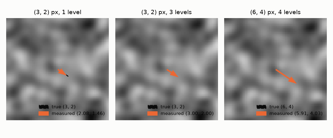
Frame B is a true crop of a larger texture moved by (dx, dy), so nothing wraps around the border. The dashed line is the true motion, the orange arrow the median flow over the 16 cells. With one level the measured flow for (3, 2) is (2.08, 1.46); with three levels it is (3.00, 2.00); a (6, 4) motion needs four levels and gives (5.91, 4.03). Command: python docs/assets/vision/make_figures.py.

Dense flow and motion mask

DenseFlow estimates the flow at every pixel with the Horn-Schunck iteration (Ziani 2025, equations 6-8); on a smooth texture moved by (0.2, 0.1) px, with intensities times 255, the endpoint error is 0.084 px. MotionMask takes the flow field and returns the pixels that move with respect to the global motion; on a synthetic flow field with a 12 by 12 square moving by an extra (2.0, 2.0), n_sigmas=3.0 and dilation=0, the IoU against the square over 20 seeds has median 0.986, minimum 0.960 and maximum 1.0.

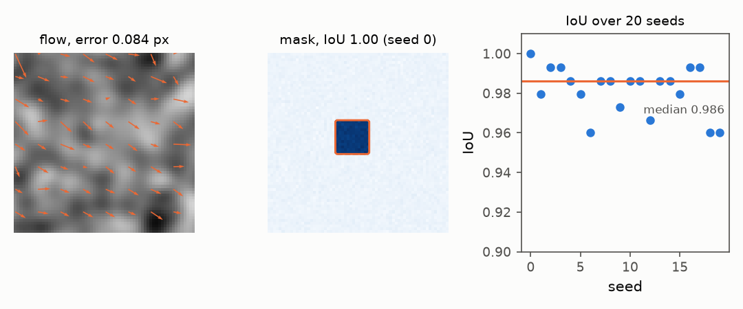
Panel (a): the flow of the texture moved by (0.2, 0.1) px, error 0.084 px. Panel (b): the mask in orange over the flow magnitude, the true square dashed, seed 0. Panel (c): the IoU for seeds 0 to 19, the median as the orange line. Command: python docs/assets/vision/make_figures.py.

API

• FrameFeatures
• DenseFlow
• MotionMask