One-Class SGD (SONAR)

One-Class SGD learns where the normal readings are and draws a boundary around them. For every new reading it gives back a number: negative means inside the boundary (normal), positive means outside (strange), and the bigger the number, the further outside. It learns one reading at a time, so it can follow the robot while it works.

One-Class SGD learns a boundary around the healthy joint residual and scores each new sample by its signed distance from that boundary. In a control loop it answers one question per reading: does this residual look like the healthy run, or does it fall outside the region the detector has learned to call normal?

1. What it is

The healthy residuals of a robot joint cluster around zero. When the payload changes, or a joint wears, the residuals move outside that cluster. A One-Class SVM finds the smallest region of the joint space that contains the healthy cluster, with the boundary at a fixed margin from the cluster's edge. A new sample is flagged when it falls outside.

The classical One-Class SVM has two problems for a control loop. First, it needs the whole healthy dataset in memory: the kernel expansion uses every training point. Second, it uses a kernel that maps the data into an infinite-dimensional space, so a plain gradient step would need the full Gram matrix at every update.

SONAR fixes both. It replaces the kernel with random Fourier features (RFF), a finite d-dimensional approximation of the RBF kernel, so each gradient step depends only on the current sample. It also adds a strongly convex regularisation to the objective, which turns the SGD convergence into a 1/T guarantee instead of the slower 1/sqrt(T) of the plain formulation. The resulting algorithm is called SONAR: SGD-based One-Class Novelty detection with Approximate RBFs.

2. How it works

The objective, from Suk and Kpotufe (2025), equation 9, is

F(w, rho) = (||w||^2 + rho^2) / 2 - nu * rho + E[ max(0, rho - w^T z(x)) ]

where w is the hyperplane normal, rho is its offset, z(x) is the RFF embedding of the sample, and nu is the expected fraction of outliers, in (0, 1). The first two terms are the strongly convex regulariser that keeps the solution well-behaved; the last is the hinge loss on the healthy samples, which pushes them inside the boundary.

The RFF embedding, from Rahimi and Recht (2007), is a cos-sin pair:

z(x) = sqrt(2/d) * [sin(omega_1^T x), cos(omega_1^T x), ..., sin(omega_d^T x), cos(omega_d^T x)]

with the frequencies omega_j drawn from N(0, 2 * gamma * I). With enough features, the dot product z(x)^T z(y) approximates the RBF kernel exp(-gamma * ||x - y||^2).

The SGD step, from Algorithm 1 of the paper, is

Z_t   = 1{ w_{t-1}^T z(X_t) <= rho_{t-1} }
w_t   = w_{t-1} - eta_{t-1} * (w_{t-1} - z(X_t) * Z_t)
rho_t = rho_{t-1} - eta_{t-1} * (rho_{t-1} - nu + Z_t)

with eta_t = step / t. Each sample updates the boundary by a small amount, so the detector learns as it goes.

The score of a sample is the signed distance from the boundary:

score(x) = rho - w^T z(x)

Positive means the sample is outside the boundary (anomalous), negative means inside (normal). The class flag threshold defaults to 0.0: any point on the wrong side of the boundary is flagged.

3. Smallest example

import numpy as np
from dense_armor.utility.anomaly.ocsvm import OneClassSGD

rng = np.random.default_rng(0)
det = OneClassSGD(n_features_rff=64, nu=0.05, n_init=50, seed=0)

for _ in range(2000):
    det.learn_one({
        "a": float(rng.normal(0.5, 0.05)),
        "b": float(rng.normal(0.5, 0.05)),
    })

print(f"healthy   {det.score_one({'a': 0.5, 'b': 0.5}):+.4f}")
print(f"anomaly   {det.score_one({'a': 5.0, 'b': 5.0}):+.4f}")

healthy   -0.0013
anomaly   +0.0088

The healthy point lies just inside the boundary: its signed distance is slightly negative (-0.0013). The anomaly lies outside: its score is positive (+0.0088). OCSVM returns a signed distance, not a probability, so the numerical contrast is small even when the two points are on opposite sides of the boundary.

4. On a real arm

The residual of joints 1-4 on a SyntheticArm payload fault. The fault (5 kg added at t = 2 s) shifts the residual on joints 1-5 by tens of N·m.

from pathlib import Path
from dense_armor.utility.anomaly.ocsvm import OneClassSGD
from dense_armor.utility.datasets import SyntheticArm

ds = SyntheticArm(
    Path("test/fixtures/urdf/panda.urdf"),
    period_s=2.0, rate_hz=50.0, n_cycles=2,
    fault_at_s=2.0, fault="payload", payload_mass=5.0,
    noise_std=(1e-3, 5e-3, 5e-2), seed=0,
)

det = OneClassSGD(feature_keys=["r0", "r1", "r2", "r3"], seed=0)

for sig, _ in ds.stream():
    q, qd, qdd = ds.trajectory(sig.t)
    tau_nom = ds.nominal_torque(q, qd, qdd)
    x = {f"r{j}": float(sig[f"tau_{j}"] - tau_nom[j]) for j in range(4)}
    _ = det.score_one(x)
    _ = det.learn_one(x)

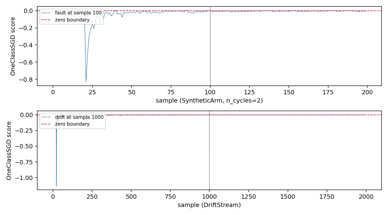
Top: SyntheticArm with n_cycles=2 (200 samples, 100 healthy, 100 fault). Bottom: DriftStream with one sudden drift at half. The boundary separates the fault on both streams: the score of the faulty samples is above the adaptive 0.95-quantile threshold from the very first post-fault sample.

5. Convergence

The paper proves (Lemma 5, Theorem 6, Corollary 7) that the distance between the SGD iterate and the population minimiser shrinks like 1/T, and Lemma 5 gives the explicit schedule eta_t = 1/t that makes the bound hold. The default step=1.0 of the detector reproduces exactly that schedule.

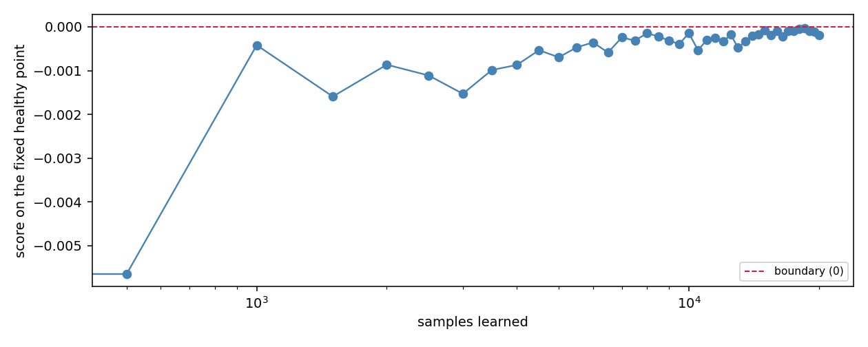
The score on one fixed healthy point, plotted against the number of samples learned. Before n_init the detector returns zero: it is still collecting the standardisation statistics. After that the score oscillates around a value that slowly moves toward its asymptotic position.

6. Numbers

SyntheticArm (200 samples, 100 healthy, 100 fault) and DriftStream (2000 samples, one sudden drift at half), every detector built with its defaults.

Stream	Protocol	ROC-AUC	False alarms on the healthy part	Threshold at the last healthy sample
SyntheticArm	learn-on-healthy	0.856	0.010	-0.0008
SyntheticArm	learn-on-all	0.671	0.010	-0.0008
DriftStream	learn-on-healthy	0.987	0.054	-0.0002
DriftStream	learn-on-all	0.769	0.054	-0.0002

The default step of 1.0 reproduces the paper's schedule eta_t = 1/t: the boundary moves on every healthy sample and the fault is separated on both streams. The default threshold of None uses the 0.95 quantile of the last 500 scores; while fewer than 50 scores have been seen the effective threshold is 1e9 and nothing is flagged.

The arm run has 100 healthy samples: after n_init = 20 they give 80 SGD steps, not the few thousand the paper's experiments use, and the ROC-AUC is 0.856. On DriftStream the 1000 healthy samples before the drift give the boundary enough updates to reach 0.987. SONAR is included here because its guarantee is the strongest of the five detectors — it is the only one with a formal bound on both Type I and Type II errors — and because when the healthy stream is long enough the separation is crisp.

Details

Where the rules come from

Suk and Kpotufe (2025) introduce SONAR in the context of one-pass non-stationary outlier detection. Equation 9 is the objective, Algorithm 1 is the SGD update, Lemma 5 and Theorems 3, 4, 6, 8 are the theoretical guarantees on the Type I and Type II errors of the final iterate. The RFF embedding is from Rahimi and Recht (2007).

The standardisation and the threshold rule are this module's choices; the paper assumes the data lie on the unit sphere, but that is a hypothesis on the data, not a preprocessing step.

Choices stated explicitly

• Standardisation. The paper assumes the RBF kernel's data lie on the unit sphere. This module standardises each feature with running mean and standard deviation, learned from the first n_init samples and frozen afterwards. Dividing each sample by its Euclidean norm, the alternative, maps a large fault in the same direction as a healthy sample onto the same point, and cannot be used.
• RFF feature count. A hyper-parameter n_features_rff (default 128). The paper's bound on the number of features (Appendix A) depends on the dimension and the assumed margin; this module does not use it as a formula.
• Step size. eta_t = step / t, with step a user constant. 1.0 recovers the paper's eta_t = 1/t; the paper's own experiments use AdaGrad.
• Embedding. The prefactor sqrt(2/d) is the one printed by Suk and Kpotufe (Section 3). With d cos-sin pairs it gives ||z(x)||^2 = 2 and z(x)^T z(y) approximates 2 K(x, y), while the paper states z(x)^T z(y) = K(x, y) in expectation; for d = 1 the printed prefactor gives z^T z = 2 where that identity needs 1. The implementation keeps the printed prefactor. With the prefactor sqrt(1/d), which gives z(x)^T z(y) close to K(x, y), the benchmark ROC-AUC (learn-on-healthy) moves from 0.856 to 0.871 on SyntheticArm and from 0.987 to 0.972 on DriftStream, so the printed prefactor stays.
• Threshold. Default None: the detector uses the 0.95 quantile of the last 500 scores, with 1e9 while fewer than 50 scores have been seen. A single float can be passed instead (e.g. 0.0, the signed distance from the boundary).

Measured cost

At the benchmark defaults (n_features_rff=128, n_init=20), on one CPU thread:

• 0.131 ms per sample for learn_one + score_one on the arm stream;
• memory flat: two 2 * n_features_rff vectors, independent of the stream length.

The budget_s declared by the class is 0.001 s.

What the detector does not do

It does not adapt quickly. The kernel approximation is fixed at construction: if the healthy distribution moves, the standardisation becomes stale and the boundary must be re-learned from scratch. For non-stationary streams the paper proposes SONARC, a variant with change-point detection and restarts; this module does not implement it.

OnlineRobustMahalanobis is the alternative when the fault is a shift of the mean and the healthy stream is short.