Linear models: first-order online optimization for streaming regression and classification¶

These are two fundamental prediction tools designed to learn from data one example at a time, without needing a huge offline database. One predicts continuous real numbers by minimizing squared errors, while the other calculates binary probabilities to tell which of two answers is more likely, and how each one learns depends on the optimizer you plug into it.

LinearRegression and LogisticRegression are the two supervised models of the package. Both fit a linear function one sample at a time, and both take any optimizer from dense_armor.utility.optim as the whole learning rule. This page shows the two models, the shape of the input they expect, and the difference between them.

1. What they do¶

A linear model predicts a target with a weighted sum of its inputs. The weights are updated one sample at a time, by the optimizer. LinearRegression predicts a real number and is trained on the squared loss; LogisticRegression predicts the probability of a binary class and is trained on the log loss.

The two models share the same body:

z = w . x
y_hat = z                        for LinearRegression
y_hat = 1 / (1 + exp(-z))        for LogisticRegression
w_next = optimizer( w, gradient of the loss at (x, y) )

w are the weights, x the input features, y the target. The model itself does not contain a learning rate: the optimizer does. Changing the optimizer changes the whole trajectory of the fit; changing l2 adds a ridge term to both models; changing intercept decides whether the model learns a bias term or is forced through the origin.

A small example with LinearRegression, SGD(lr=0.5), no intercept, three samples of the line y = 3 * x:

reg = LinearRegression(optimizer=SGD(lr=0.5), intercept=False)
for _ in range(50):
    reg.learn_one({"x": 1.0}, 3.0)
    reg.learn_one({"x": 2.0}, 6.0)
    reg.learn_one({"x": 3.0}, 9.0)
reg.predict_one({"x": 1.0})  # 3.0000

The weight reaches 3.0 after enough passes, exactly the slope of the line. The same body with LogisticRegression on a two-feature problem that is linearly separable learns to separate the classes:

clf = LogisticRegression(optimizer=Adam(lr=0.1), intercept=True)
for _ in range(200):
    clf.learn_one({"a": 1.0, "b": 0.5}, 1)
    clf.learn_one({"a": -1.0, "b": -0.5}, 0)
clf.predict_proba_one({"a": 1.0, "b": 0.5})   # {0: 0.0013, 1: 0.9987}
clf.predict_proba_one({"a": -1.0, "b": -0.5}) # {0: 0.9987, 1: 0.0013}

The probabilities are symmetric around 0.5: the model separates the two classes with the same confidence on both sides.

2. The input shape¶

Both models read a dict at every sample. The keys of the dict are the feature names; the values are the numeric features; the target is passed separately as the second argument of learn_one. The first sample fixes the order of the features: either the explicit feature_keys argument, or the sorted keys of the first dict. Subsequent samples must have the same keys.

import numpy as np
from dense_armor.utility.optim import SGD
from dense_armor.utility.linear.glm import LinearRegression

reg = LinearRegression(optimizer=SGD(lr=0.1), intercept=False,
                       feature_keys=["x"])
state = reg.init_state(1)
state, out = reg.step(state, {"x": np.asarray(1.0),
                              "y": np.asarray(3.0)})
print(out)

0.0

The pure form takes the same dict, with the target under the key "y". The output is the prediction on the current sample, before the update.

A None or a non-numeric value on any feature is counted in n_missing and the sample is skipped, without raising. This keeps the loop alive on a stream with missing rows.

3. The learning rate¶

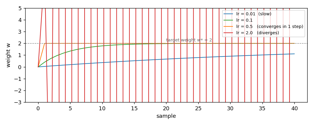
The learning rate belongs to the optimizer, not to the model. The figure shows four runs of LinearRegression(intercept=False) on the same one-feature problem, target weight w* = 2, each with SGD at a different lr:

Trajectory of the weight for four learning rates

`lr`	weight after 1 step	after 10	after 30	after 60
`0.01`	`0.0400`	`0.3659`	`0.9090`	`1.4049`
`0.1`	`0.4000`	`1.7853`	`1.9975`	`2.0000`
`0.5`	`2.0000`	`2.0000`	`2.0000`	`2.0000`
`2.0`	`8.0000`	`-118096.0000`	`-4.1e14`	`-8.5e28`

lr = 0.5 reaches the target in a single step, because for a one-feature quadratic loss the update w -= lr * 2 * (w - w*) reaches w* exactly when lr = 0.5. lr = 2.0 diverges: the same formula has a factor (1 - 2 lr) = -3, whose absolute value is larger than one.

The safe range of lr depends on the curvature of the loss, not on the model. With several features, the largest eigenvalue of the covariance matrix sets the upper bound. A smaller lr is safer, at the cost of slower convergence.

4. On a real arm¶

A SyntheticArm from a real Panda URDF gives q, qd, and tau at 50 Hz. The same LinearRegression learns the torque of joint 0 as a function of its velocity, with three different optimizers:

from pathlib import Path
import numpy as np
from dense_armor.utility.datasets import SyntheticArm
from dense_armor.utility.linear.glm import LinearRegression
from dense_armor.utility.optim import SGD, AdaGrad, Adam

for opt, lr in [(SGD(lr=1e-3), 1e-3), (AdaGrad(lr=10.0), 10.0),
                (Adam(lr=0.5, beta1=0.99), 0.5)]:
    ds = SyntheticArm(Path("test/fixtures/urdf/panda.urdf"),
                      period_s=1.0, rate_hz=50.0, n_cycles=2, seed=0)
    reg = LinearRegression(optimizer=opt, intercept=True,
                           feature_keys=["qd0"])
    for sig, _ in ds.stream():
        reg.learn_one({"qd0": float(sig["qd_0"])}, float(sig["tau_0"]))
    pred = round(reg.predict_one({"qd0": 0.5}), 3)
    print(type(opt).__name__, pred)

SGD -2.158
AdaGrad -2.824
Adam -4.999

SGD and AdaGrad converge to the same neighbourhood. Adam on the same 100-sample stream with the same parameters moves further: it carries two running averages instead of one, and on 100 samples it has not settled yet. With more samples (400) and a longer memory beta1=0.99, Adam converges to -2.273. The choice of optimizer is what changes the trajectory; the model is the same three lines of code.

Details¶

References¶

The two models are standard: the squared loss and its gradient 2 (y_hat - y) x, the log loss and its gradient (sigmoid(z) - y) x. They are the textbook models, and no paper is needed to derive them. The learning rule is entirely delegated to the optimizer; the list of sources for the optimizers is in the optim/ pages.

The l2 term adds l2 * w to the gradient of both models. This is the ridge regularization of Hoerl and Kennard (1970).

Choices stated explicitly¶

Feature order fixed on the first sample. The model remembers the order of the keys it saw, either from the feature_keys argument or from the sorted keys of the first dict. Every later sample must use the same keys.
intercept=True by default. The model prepends a constant 1 to the features and learns a bias term together with the weights. Set intercept=False when the problem is known to pass through the origin and the bias should be suppressed.
Missing values counted, not raised. A None, a string, or any non-numeric value on a feature makes the sample count in n_missing and be skipped. learn_one(None, y) does the same. This keeps a loop over a real stream alive when the input has holes.
Pure form returns the prediction before the update. The pair init_state(dim) and step(state, v) returns the new state and the prediction on the current sample, computed with the weights the model had before seeing the label. This matches the streaming semantics: the model predicts first, then learns.

Measured cost¶

On one CPU thread, LinearRegression with two features and SGD, the median of 1000 samples after a warm-up of 200 is 0.0139 ms per sample, including predict_one and learn_one. The cost is dominated by the matrix-vector product and the outer product, not by the optimizer.

Development diary¶

This is the first page that documents two models on the same file. The shared body (feature resolution, intercept handling, missing-value skipping, pure form) is stated once, in Section 2. The two optimizers used in the examples (SGD, Adam) were chosen because they cover the two ends of the first-order spectrum: fixed step and adaptive. The three optimizer columns in Section 4 come from the same script that runs the comparison table in docs/optim/index.md, so the values here are the same as the values there. The figure was regenerated after the first attempt placed the script in the wrong directory and the sys.path insertion did not reach the package.