Bayesian linear regression: closed-form sequential posterior estimation

A standard prediction tool gives you a single number, guessing the outcome but hiding how sure it actually is. This tool learns one example at a time in closed form, returning both a prediction and a range around it: the range stays wide where data is scarce and shrinks where examples are abundant, giving a control system a measure of confidence.

BayesianLinearRegression is the Bayesian companion of LinearRegression. It learns the same linear function on the same stream, but it returns not a single prediction, it returns an interval. The width of the interval grows where the model has seen few samples and shrinks where the model has seen many, which is the kind of uncertainty that a frequentist model does not give. This page shows the update, the two equivalent forms (streaming and batch), and the predictive interval on a real stream.

1. What it does

On each sample the model updates a Gaussian posterior over the weights. The posterior is fully described by two quantities: a mean m, which is the current best guess of the weights, and a covariance S, which is the current uncertainty on that guess. The updates are:

A_t = A_{t-1} + beta * x_t x_t^T
b_t = b_{t-1} + beta * x_t y_t
m_t = S_t @ b_t
S_t = inv(A_t)

with A_0 = alpha * I, b_0 = 0. alpha is the prior precision on the weights, beta the precision of the noise on the targets. The prediction on a sample x is the posterior mean at x, and the predictive variance is 1/beta + x^T S x.

A small example. Suppose the model has seen five samples of the line y = 2 x and the current m is roughly [2.0], S is small. On a new sample x = 1.0 the prediction is around 2.0 with a narrow interval. On a sample x = 50.0, far outside the observed range, the same m predicts a value around 100.0 but the interval is wide, because the model has never seen x near 50 and cannot be sure that the linear relation still holds.

The model is closed-form: no optimizer, no learning rate, no iteration. The alpha and beta hyper-parameters set the prior and the noise model, not the speed of convergence.

2. The two forms

The object form updates the posterior one sample at a time:

import numpy as np
from dense_armor.utility.linear.bayes import BayesianLinearRegression

model = BayesianLinearRegression(alpha=1.0, beta=1.0,
                                 intercept=False, feature_keys=["x"])
for i in range(5):
    model.learn_one({"x": float(i + 1)}, float(2 * (i + 1)))
print(round(model.predict_one({"x": 3.0}), 3))

5.893

Unlike LinearRegression and LogisticRegression, this estimator does not expose a pure init_state / step pair. The Bayesian update is not a gradient step: it is a closed-form update of the posterior, and it is not used inside jax.lax.scan by the rest of the package. The estimator runs through learn_one only.

The streaming update is algebraically identical to the batch posterior: on the same stream the two produce the same m and the same S up to numerical precision (max|dm| ~ 1e-16, max|dS| ~ 1e-19 on a 20-sample test). The tests in test/linear/test_bayes.py check this equivalence.

3. The predictive interval

The predictive variance on a sample x is 1/beta + x^T S x. The first term is the noise on the target, the second is the uncertainty on the weights projected onto x. The second term grows with x^T S x, which is small where the model has seen data and large elsewhere.

The figure shows the posterior mean and the mean +/- 2 std band after ten samples of a noisy line, on a range that goes beyond the observed samples:

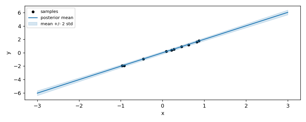
The band is narrow around the observed samples and wide at the two ends. That is the Bayesian signature: the model admits it does not know.

predict_one(..., return_estimate=True) returns the mean and the standard deviation of the prediction as a single named tuple, without a second call:

from dense_armor.utility.linear.bayes import BayesianLinearRegression

model = BayesianLinearRegression(alpha=1.0, beta=1.0,
                                 intercept=False, feature_keys=["x"])
for i in range(5):
    model.learn_one({"x": float(i + 1)}, float(2 * (i + 1)))
out = model.predict_one({"x": 3.0}, return_estimate=True)
print(round(out.mean, 3), round(out.std, 6))

5.893 1.077365

The standard deviation 1.077 is what the model believes about the prediction on x = 3 after five samples with alpha = beta = 1. The value is large because the prior is loose and the noise is large. With more samples, or a larger beta, the interval shrinks. On a far away x the same number would be much larger. This is the object the caller can use to decide whether to trust the prediction, something LinearRegression cannot provide.

4. On a real arm

A SyntheticArm from a real Panda URDF gives q, qd, and tau at 50 Hz. The model learns the torque of joint 0 as a function of its velocity:

from pathlib import Path
import numpy as np
from dense_armor.utility.datasets import SyntheticArm
from dense_armor.utility.linear.bayes import BayesianLinearRegression

ds = SyntheticArm(Path("test/fixtures/urdf/panda.urdf"),
                  period_s=1.0, rate_hz=50.0, n_cycles=2, seed=0)
model = BayesianLinearRegression(alpha=1.0, beta=100.0,
                                 intercept=True, feature_keys=["qd0"])
for sig, _ in ds.stream():
    model.learn_one({"qd0": float(sig["qd_0"])}, float(sig["tau_0"]))
print(round(model.predict_one({"qd0": 0.5}), 3))

8.041

The value 8.041 is the posterior mean on qd = 0.5. It is not close to the -2.158 of SGD(lr=1e-3) on the same stream, and the gap is not a bug. The reason is that the two methods answer two different questions.

SGD with lr=1e-3 has not converged after 100 samples: its weight w = [1.43, -7.18] is still far from the least-squares optimum of this stream. BayesianLinearRegression solves the same least-squares problem in closed form, and its posterior mean [8.19, -0.294] is the exact solution for the given alpha, beta. The first component is the bias term, and it is very close to the target mean mean(tau_0) = 8.19 of this stream: the joint torque has a large constant offset and a small dependence on the velocity, so any correctly fitted model will put most of the prediction in the bias.

Which one is the right tool? It depends on the question:

• To track a changing relationship on a long stream, first-order optimizers (SGD, AdaGrad, Adam) are the right tool, because they adjust the weights sample by sample.
• To obtain a closed-form estimate together with its uncertainty on a stationary window, BayesianLinearRegression is the right tool, because it does not need a learning rate and it gives an interval, not a point.

Neither is better in the abstract: they answer different questions.

Details

References

Bishop, C. M. (2006). Pattern Recognition and Machine Learning. Springer. Section 3.3.1, equation 3.53, page 152:

m_N = beta * S_N * Phi^T t
S_N^{-1} = alpha * I + beta * Phi^T Phi

The docstring of bayes.py derives the streaming form m_N = m_{N-1} + K (y - x^T m_{N-1}) from equation 3.53 by direct algebra, and the tests compare the two. Section 3.3.1, lines after equation 3.51, states explicitly: "if data points arrive sequentially, then the posterior distribution at any stage acts as the prior distribution for the subsequent data point". This implementation follows that statement.

Choices stated explicitly

• Zero-mean isotropic prior. The prior on the weights is N(0, alpha^{-1} I). This is the special case that Bishop uses in the remainder of Section 3.3 after equation 3.52. A general Gaussian prior N(m_0, S_0) is handled by the batch form, not by the streaming form.
• Closed-form update. The mean and covariance are updated in closed form at every sample. No optimizer is involved. The alpha and beta parameters are the same ones in Bishop, not a learning rate.
• Symmetrisation of the covariance. After the rank-one update of S the code symmetrises it: S = 0.5 (S + S^T). Without this, numerical drift can break the symmetry after many samples and the Kalman update can become unstable.
• return_estimate=True returns an Estimate. The object has attributes .mean and .std. This is the caller's window on the posterior uncertainty, and it is the reason the model is useful for applications where the prediction alone is not enough.
• return_std=True returns the standard deviation alone. For callers that only need the width of the interval, without the mean.
• No pure init_state / step form. The estimator is used through learn_one only. The Bayesian update is closed form and does not need the jax.lax.scan machinery.

Measured cost

The covariance is a d x d matrix, one entry per pair of features. On a problem with d = 100, the update is the most expensive of the models in the package. On the two-feature problem of the tests, the update is 0.0178 ms per sample, close to AdaGrad.

Development diary

The docstring was verified against Bishop Section 3.3.1, equation 3.53 on page 152, extracted from the PDF via pypdf during this session. The streaming update in the docstring matches the batch form of Bishop step by step. The example in Section 4 was rewritten after an initial version compared the prediction to SGD on the same stream and reported a "discrepancy"; the discrepancy was not a bug, it was a comparison between an exact closed-form solution and a stochastic method that has not yet converged, and the page now says so explicitly. The figure was regenerated to show the interval, not just the mean.