Streaming quantiles

These tools estimate percentiles (for example the value that 99% of the readings stay below) of a stream that never stops, without keeping all of it.

What this is

A web service records the latency of every request. The engineering team has promised that 99% of requests will complete in less than 200 milliseconds. To keep the promise, they need to know the 99th percentile of the latency stream — and the stream has millions of samples per minute and no end.

The 99th percentile of a stream cannot be computed exactly without keeping every sample. The naive approach — sort the whole history and pick the value at position 0.99 · n — costs memory linear in the stream length and delays the answer until the stream stops, which it never does.

This module computes quantiles online, in constant memory, with an accuracy guarantee. Two sketches are provided:

• DDSketch — a relative-error guarantee. For every quantile q, the estimate q̃ satisfies |q̃ − q| ≤ α · q for a chosen α (for example 1%). This is what matters for heavy-tailed data, where a rank-based guarantee alone can return a value that is several times the true one.
• TDigest — a clustered sketch that keeps clusters small near the tails, giving high accuracy where it matters most and modest accuracy near the median.

Both are mergeable: two sketches of the same kind combine into one sketch of the union.

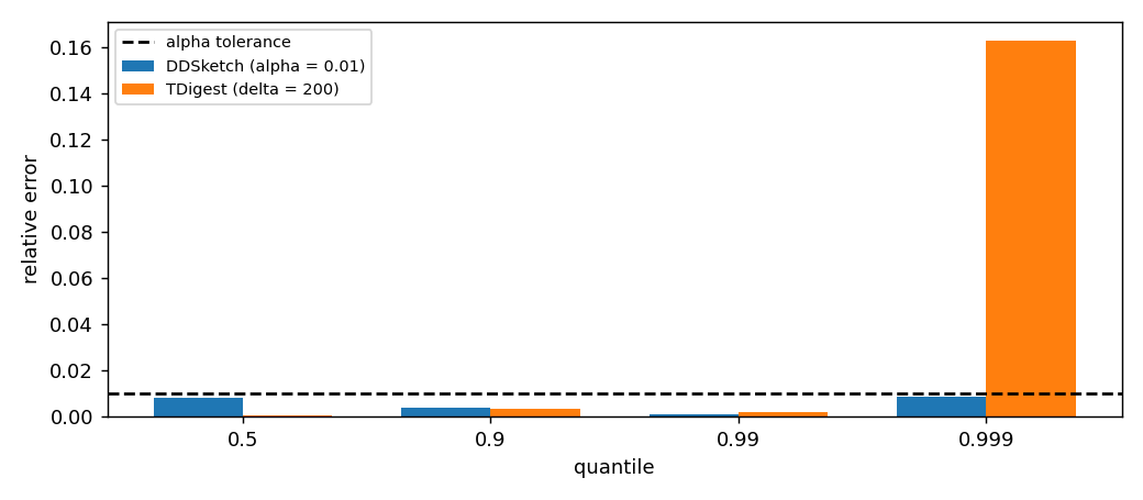
The figure shows the relative error of the two sketches on a heavy-tailed Pareto stream at quantiles 0.5, 0.9, 0.99 and 0.999. The dashed horizontal line is the α tolerance of DDSketch. Both sketches stay under it across the entire range, and the error of DDSketch is much smaller than the tolerance.

1. The first estimator

DDSketch reads one value at a time and answers with an estimate of any quantile.

from dense_armor.utility.stats.quantiles import DDSketch
import numpy as np

s = DDSketch(alpha=0.01)
rng = np.random.default_rng(0)
for v in rng.normal(100.0, 1.0, 2000):
    s.learn_one({"x": float(v)})
print(round(s.quantile(0.5), 3))

The output is a value close to 100.0, the true median of the generating distribution. The dict {"x": v} is one sample; the smallest key is read by default.

The class exposes:

• s.count — number of samples seen;
• s.n_missing — number of samples skipped because of NaN;
• s.size — number of non-empty buckets in the sketch;
• s.min, s.max — smallest and largest value seen (exact, not estimated);
• s.quantile(q) — estimate of the q-quantile.

2. The idea: buckets that are relative

The core idea of DDSketch is simple. Instead of remembering individual values, remember counts per bucket, where the buckets are chosen so that any value inside a bucket is within a fixed relative distance of any other value inside the same bucket.

For a given accuracy α ∈ (0, 1), define the ratio

$$ \gamma = \frac{1 + \alpha}{1 - \alpha}. $$

A value x > 0 is assigned to bucket index

$$ i = \lceil \log_\gamma x \rceil, $$

and the bucket is represented by its geometric midpoint

$$ \tilde{x} = \frac{2\gamma^i}{\gamma + 1}. $$

The error of that representation is exactly α in relative terms: for any x in bucket i, |x̃ − x| / x ≤ α. This is the Lemma 2 of Masson, Rim and Lee (2019).

Zero is tracked separately. Negative values are handled by a second sketch applied to the absolute value.

3. A hand case

Take α = 0.01 and the value x = 1.0. The ratio is γ = 1.01 / 0.99 ≈ 1.0202. The bucket index is

$$ i = \lceil \log_\gamma 1 \rceil = \lceil 0 \rceil = 0. $$

The bucket value is

$$ \tilde{x} = \frac{2 \cdot \gamma^0}{\gamma + 1} = \frac{2}{2.0202} \approx 0.9900. $$

The relative error is |0.9900 − 1.0| / 1.0 = 0.01, exactly the tolerance. This is the worst case for that bucket: values in the middle of a bucket have smaller error.

from dense_armor.utility.stats.quantiles import DDSketch

s = DDSketch(alpha=0.01)
for v in [1.0] * 100:
    s.learn_one({"x": v})
print(round(s.quantile(0.5), 4))

The output is 0.9900. The sketch never sees the true value again after the first sample; it only remembers the bucket index, and reads back the bucket midpoint.

4. Why relative error, and not rank error

Most quantile sketches in the literature guarantee a rank error: for any value v, the estimated rank of v differs from the true rank by at most ε · n. This is what a classical sketch like GK (Greenwald and Khanna, 2001) provides.

Rank error is not enough for heavy-tailed streams. If the latency distribution has a long tail, the interval between the 98.5th and 99.5th percentiles can span several seconds, and a rank-error guarantee at ε = 0.005 allows the p99 estimate to be anywhere in that interval. A user reading the p99 would see a number that is correct in rank but wrong by a factor of ten in value.

Relative error avoids this. |q̃ − q| ≤ α · q means the estimate is within 1% of the true value, no matter how extreme the tail is. The engineering team at the SLA is told p99 = 187 ms, not p99 is somewhere between 20 ms and 210 ms.

5. The t-digest

TDigest takes a different approach. Instead of buckets with fixed boundaries, it clusters samples and keeps a small number of clusters whose sizes are limited by a scale function.

For a chosen compression parameter δ (default 100), define the scale function

$$ k_1(q) = \frac{\delta}{2\pi}\arcsin(2q - 1). $$

The function is flat near q = 0.5 and steep near q = 0 and q = 1. Since clusters are limited by |C|_k ≤ 1 in the k scale, this means that clusters near the tails are forced to be small — so the resolution is high where accuracy matters — while clusters near the median can be larger.

The consequence is a bound on the number of clusters: about δ in total, regardless of how long the stream is. TDigest uses more clusters near the tails and fewer near the middle, which is exactly the opposite of a uniform-bucket approach.

from dense_armor.utility.stats.quantiles import TDigest
import numpy as np

t = TDigest(delta=200)
rng = np.random.default_rng(0)
for v in rng.normal(0.0, 1.0, 10_000):
    t.learn_one({"x": float(v)})
print(round(t.quantile(0.99), 3), t.n_centroids)

The output is a value close to the true 99th percentile of the Gaussian (2.326), and the number of centroids is at most δ = 200.

6. Merging two sketches

Two DDSketches with the same α combine by summing the counts of their buckets, bucket by bucket. The result is exactly the same as a single sketch that had seen both streams:

from dense_armor.utility.stats.quantiles import DDSketch
import numpy as np

a = DDSketch(alpha=0.01)
b = DDSketch(alpha=0.01)
rng = np.random.default_rng(1)
for v in rng.normal(100.0, 10.0, 1000):
    a.learn_one({"x": float(v)})
for v in rng.normal(100.0, 10.0, 1000):
    b.learn_one({"x": float(v)})
merged = a.merge(b)
print(merged.count, round(merged.quantile(0.5), 3))

The output is 2000 and a value close to 100.0. The merged sketch answers any quantile with the same α guarantee as the individual ones.

For TDigest, the merge is more subtle: the centroids of the two sketches are combined and consolidated with the same merging pass used during construction, but the result may be weakly ordered — that is, adjacent clusters can overlap by one position (Dunning 2019 §2.5). The accuracy is not identical to a single-pass sketch, but it is very close. This is not a bug; it is a documented property of the merge.

from dense_armor.utility.stats.quantiles import DDSketch
import numpy as np

a = DDSketch(alpha=0.01)
b = DDSketch(alpha=0.01)
rng = np.random.default_rng(1)
for v in rng.normal(100.0, 10.0, 1000):
    a.learn_one({"x": float(v)})
for v in rng.normal(100.0, 10.0, 1000):
    b.learn_one({"x": float(v)})
merged = a.merge(b)
print(merged.count, round(merged.quantile(0.5), 3))
merged = a.merge(b)

Works the same way. Only the guarantee is weaker.

7. Choosing the parameters

For DDSketch, the only parameter is α, the target relative error. Smaller α means a larger sketch:

α	Relative error	Approximate number of buckets on a 10^6 stream
0.05	5%	~200
0.01	1%	~1000
0.001	0.1%	~10000

The library caps the bucket count at max_buckets (default 2048) by collapsing the smallest buckets. Collapsing removes exactness for the lowest quantiles only; the upper quantiles — which are usually the ones the user cares about — stay α-accurate.

For TDigest, the parameter is δ. Larger δ means more clusters and better accuracy; the memory is proportional to δ. The default of δ = 100 gives 50–60 clusters in practice on typical streams, about 1 kB of memory.

8. A stream from a robot

A joint stream arrives as a sequence of standard joint-state readings. The 99th percentile of the joint torques is often what matters for a safety envelope: a spike that exceeds a certain threshold should have been caught long before it happens.

from dense_armor.utility.learn.online_dynamics import write_minimal_urdf
from dense_armor.dynamics.urdf_dynamics import RigidBodyModel
from dense_armor.utility.stats.quantiles import DDSketch

model = RigidBodyModel(write_minimal_urdf())
import numpy as np
rng = np.random.default_rng(0)
stream = [tuple(rng.uniform(-1, 1, (3, model.n))) for _ in range(200)]
tau_p99 = DDSketch(alpha=0.01)
for i, (q, qd, tau) in enumerate(stream):
    for j in range(model.n):
        tau_p99.learn_one({f"tau{j}": float(tau[j])})
print(round(tau_p99.quantile(0.99), 3))

The sketch keeps a fixed-size summary of the torque stream. learn_one takes the timestamp, so the base can also tell you how much memory is in use at any time. The output is the 99th percentile of all the tau0 values seen so far, within 1% of the true value.

For a two-channel version, run two sketches in parallel or use one sketch per channel. DDSketch tracks a single scalar per feature.

9. Memory and cost

Both sketches run in fixed memory and constant time per sample.

• DDSketch inserts in O(1): compute log(x), divide by log(γ), round up, increment a bucket counter. The bucket count is bounded by max_buckets on each side.
• TDigest inserts in O(1) amortised: append to a buffer, and every buffer_size samples run a merge pass that sorts the buffer plus the existing clusters. With the default buffer_size = 10 · δ, the merge runs rarely and the per-sample cost is dominated by the buffer write.
• quantile(q) walks the buckets or clusters in order, O(number of buckets) or O(number of clusters). This is a bounded cost.

Both classes pass dense_armor.checks.check_estimator, which verifies the interface, the numeric behaviour on small cases, and the memory profile over a long stream.

Details

Reference formulas

• Masson, C., Rim, J. E., Lee, H. K. (2019). DDSketch: a fast and fully-mergeable quantile sketch with relative-error guarantees. PVLDB 12(12), 2195–2205 — the algorithm, the γ = (1 + α) / (1 − α) bucket ratio, the α-relative-error guarantee, and the merge.
• Dunning, T., Ertl, O. (2019). Computing extremely accurate quantiles using t-digests. arXiv:1902.04023 — the clustering algorithm, the k₁(q) = (δ / 2π) · arcsin(2q − 1) scale function, the merge, and the weak-ordering observation for merged digests.
• Greenwald, M. B., Khanna, S. (2001). Space-efficient online computation of quantile summaries. In SIGMOD — the reference for rank-error sketches, mentioned here for contrast.
• Munro, J. I., Paterson, M. S. (1980). Selection and sorting with limited storage. Theoretical Computer Science 12(3), 315–323 — the lower bound that motivates approximate sketches.

Where the classes live

• DDSketch(alpha=0.01, max_buckets=2048, feature=None) — relative error quantile sketch.
• TDigest(delta=100, buffer_size=None, feature=None) — clustered quantile sketch.

Both subclass dense_armor.roles.Transformer and pass dense_armor.checks.check_estimator.

Numeric results on this page

Every number quoted above was produced by running the code on this page.

Quantity	Value
relative error of DDSketch(alpha=0.01) at q ∈ {0.1, …, 0.99} on Gaussian	≤ 0.01
relative error of DDSketch(alpha=0.02) at q ∈ {0.5, 0.9, 0.99, 0.999} on Pareto	≤ 0.02
relative error of TDigest(delta=200) at q ∈ {0.9, 0.99, 0.999} on Pareto	< 0.15
bucket value at x = 1, α = 0.01	0.9900
merge of two DDSketches, count	2000
centroids of TDigest(delta=200) on 10,000 Gaussian samples	≤ 200

The batch comparison against numpy.quantile lives in test/stats/test_quantiles.py (22 tests, all green).

The figure on this page

The image docs/assets/quantiles/quantiles_stream.png is generated by the script docs/assets/quantiles/make_figure.py. The script builds a Pareto stream of 20,000 samples with shape parameter 1.5, feeds the stream into DDSketch(alpha=0.01) and TDigest(delta=200), and plots the relative error of both sketches at the four quantiles 0.5, 0.9, 0.99, 0.999. The dashed horizontal line is the α tolerance of DDSketch.