Moments¶

These tools keep the average, the wobble and a few other summary numbers of a signal, updated with every new reading, without storing the readings.

What this is¶

Imagine you are watching a single joint of a robot move. You want to know its average angle, how much it wobbles, and whether the wobble is symmetric or one-sided. You do not want to keep every reading — the robot runs for days. You want a handful of numbers that summarize what has been seen so far and update with each new reading.

That handful of numbers is what statisticians call the moments of a distribution: the mean, the variance, the skewness, the kurtosis, plus the minimum and maximum. This module computes them online, one sample at a time, in fixed memory.

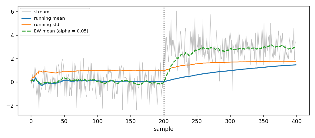
Running mean and standard deviation over a stream that steps from N(0, 1) to N(3, 1) at the middle of the trace. The EW mean (dashed) tracks the new regime faster than the running mean.

The figure shows the standard situation. A stream of 400 samples is drawn from a Gaussian distribution whose mean shifts from 0 to 3 at sample 200. The grey trace is the raw stream; the blue line is the running mean that the module computes; the red line is the running standard deviation. The dashed orange line is the exponentially weighted mean, which responds more quickly to the shift.

1. The first statistic¶

The estimator RunningMoments reads one value at a time from a dict and keeps the running mean, variance, skewness, kurtosis, minimum and maximum.

from dense_armor.utility.stats.moments import RunningMoments

m = RunningMoments()
for v in [1.0, 2.0, 3.0, 4.0, 5.0]:
    m.learn_one({"x": v})
print(m.mean, m.var)

After the five samples, m.mean is 3.0 and m.var is 2.5. The dict {"x": v} is one sample; the smallest key is read by default. The full set of properties reads:

m.count — number of samples seen;
m.mean — arithmetic mean;
m.var — sample variance with n − 1 in the denominator;
m.std — square root of var;
m.skewness — third standardized moment;
m.kurtosis — fourth standardized moment minus 3;
m.min, m.max, m.ptp — smallest, largest, and their difference;
m.n_missing — number of samples skipped because of NaN.

2. What counts as a sample¶

The input is always a dict. A specific feature can be named:

from dense_armor.utility.stats.moments import RunningMoments

m = RunningMoments()
for v in [1.0, 2.0, 3.0, 4.0, 5.0]:
    m.learn_one({"x": v})
print(m.mean, m.var)
m = RunningMoments(feature="temperature")
m.learn_one({"temperature": 21.4, "humidity": 0.6})

The value must be a number. NaN is allowed and means "this sensor missed a reading": the sample is skipped and counted in n_missing, and the running summary is left untouched. A robot with an intermittent sensor therefore does not see its average poisoned by a missing value.

from dense_armor.utility.stats.moments import RunningMoments

m = RunningMoments()
for v in [1.0, 2.0, 3.0, 4.0, 5.0]:
    m.learn_one({"x": v})
print(m.mean, m.var)
m = RunningMoments(feature="temperature")
m.learn_one({"temperature": 21.4, "humidity": 0.6})
m = RunningMoments()
for v in [1.0, float("nan"), 3.0]:
    m.learn_one({"x": v})
print(m.count, m.n_missing, m.mean)

The output is 2 1 2.0. Two valid samples, one skipped, mean of the valid samples 2.0.

3. Why the obvious formula fails¶

The mean and the variance of a set of numbers x₁, …, xₙ are

$$ \text{mean} = \frac{1}{n}\sum_{i=1}^{n} x_i, \qquad \text{var} = \frac{1}{n-1}\sum_{i=1}^{n} (x_i - \text{mean})^2. $$

There is an algebraic identity that rewrites the variance in terms of the raw sum of squares:

$$ \text{var} = \frac{1}{n-1}\left(\sum_{i=1}^{n} x_i^2 - n\,\text{mean}^2\right). $$

The temptation is to keep two running sums — sum(x) and sum(x²) — and compute the variance from them. This is a trap. When the mean is large compared to the wobble (a joint holding 90° ± 0.1°), the two numbers inside the parenthesis are nearly equal and their difference is dominated by rounding error. In extreme cases the computed variance comes out negative.

Welford (1962) gives the fix. Instead of the raw sum of squares, keep the centered second moment M2 = Σ (xᵢ − mean)² and update it incrementally. Each new sample adds a small correction that never involves cancellation. The same technique extends to the third and fourth moments, using the formulas of Pébay (2008):

$$ \begin{aligned} n &\leftarrow n + 1 \ \delta &= x - \text{mean} \ \delta_n &= \delta / n \ \text{mean} &\leftarrow \text{mean} + \delta_n \ M4 &\leftarrow M4 + \delta\,\delta_n^3\,(n - 1)(n^2 - 3n + 3) + 6\,\delta_n^2\,M2 - 4\,\delta_n\,M3 \ M3 &\leftarrow M3 + \delta\,\delta_n^2\,(n - 1)(n - 2) - 3\,\delta_n\,M2 \ M2 &\leftarrow M2 + \delta\,\delta_n\,(n - 1) \end{aligned} $$

Every symbol is a number already kept in memory: n is the sample count, mean is the running mean, M2, M3, M4 are the second, third and fourth central moments, δ is the deviation of the new sample from the current mean, and δₙ = δ / n. The update uses only additions, subtractions, multiplications and one division. No sum of squares is ever formed, so no cancellation ever occurs.

Skewness and kurtosis are read off the central moments:

$$ \text{skew} = \frac{M3/n}{(M2/n)^{3/2}}, \qquad \text{kurt} = \frac{n\,M4}{M2^2} - 3. $$

The skewness measures the asymmetry of the distribution: zero for a symmetric stream, positive when the right tail is heavier. The kurtosis measures how much the tails stick out compared to a Gaussian: zero for a Gaussian, negative for a light-tailed stream like a uniform distribution, positive for a heavy-tailed stream.

4. A hand case¶

Take the five samples [1, 2, 3, 4, 5]. After all five, the classic formulas give:

$$ \text{mean} = 3,\quad M2 = 10,\quad M3 = 0,\quad M4 = 34. $$

From those,

$$ \text{var} = M2 / (n - 1) = 10 / 4 = 2.5, $$ $$ \text{skew} = 0, $$ $$ \text{kurt} = \frac{5 \cdot 34}{10^2} - 3 = \frac{170}{100} - 3 = 1.7 - 3 = -1.3. $$

The code produces exactly these numbers:

from dense_armor.utility.stats.moments import RunningMoments

m = RunningMoments()
for v in [1.0, 2.0, 3.0, 4.0, 5.0]:
    m.learn_one({"x": v})
print(m.mean, m.var, m.skewness, m.kurtosis)

The output is 3.0 2.5 0.0 -1.3. The values agree with numpy and scipy.stats on the same data to machine precision.

5. Combining two halves¶

Two RunningMoments built on disjoint halves of a stream can be merged into the summary of the union. The merged summary is exactly the same as the one a single accumulator would have produced from both halves together, not an approximation. The formulas are those of Chan, Golub and LeVeque (1979) for the variance, extended by Pébay (2008) to the third and fourth moments.

from dense_armor.utility.stats.moments import RunningMoments

m = RunningMoments()
for v in [1.0, 2.0, 3.0, 4.0, 5.0]:
    m.learn_one({"x": v})
print(m.mean, m.var, m.skewness, m.kurtosis)
left = RunningMoments()
right = RunningMoments()
for v in [1.0, 2.0, 3.0]:
    left.learn_one({"x": v})
for v in [10.0, 20.0]:
    right.learn_one({"x": v})
merged = left.merge(right)
print(merged.count, round(merged.mean, 3))

The output is 5 7.2. The merged count is the sum of the two, and the merged mean is (1 + 2 + 3 + 10 + 20) / 5 = 7.2, the mean of the union.

This is how a sharded system computes one global statistic without ever moving the samples. Each worker builds a summary of its own data, the workers send their summaries to a coordinator, and the coordinator merges them. The network cost is the size of one summary per worker, which is fixed regardless of how many samples each worker saw.

6. All joints at once¶

A robot has many joints. Feeding them one by one into separate RunningMoments objects works, but is repetitive to write and easy to get wrong. RunningMomentsVector keeps one RunningMoments per channel and updates all of them from a single dict.

from dense_armor.utility.stats.moments import RunningMomentsVector

v = RunningMomentsVector()
for q in ([0.1, 0.2], [0.11, 0.19], [0.09, 0.21]):
    v.learn_one({"q0": q[0], "q1": q[1]})
summary = v.transform_one({})
print(round(summary["q0"]["mean"], 4), round(summary["q1"]["mean"], 4))

The output is 0.1 0.2. Both channels move through the tracker in lockstep, which is exactly what a synchronised joint stream looks like. The channel order is the sorted keys of the first dict seen, or the explicit list passed as features=[...].

RunningMomentsVector.merge combines two vector summaries channel by channel, using the same exact pairwise formulas.

7. Following a drift¶

Averaging over the whole history is the wrong answer when the world drifts. A robot picks up a payload, a sensor warms up, a network changes: the old samples describe a regime that no longer exists.

EWStats weights recent samples more. The running mean becomes

$$ \text{mean}t = (1 - \alpha)\,\text{mean}{t-1} + \alpha\, x_t, $$

where α is a number between 0 and 1 called the forgetting factor. The variance follows West (1979) so it also forgets. α = 1 copies the last value; α = 0.05 corresponds roughly to averaging over the last twenty samples.

from dense_armor.utility.stats.moments import EWStats

e = EWStats(alpha=0.05)
for _ in range(500):
    e.learn_one({"x": 1.0})
for _ in range(500):
    e.learn_one({"x": 5.0})
print(round(e.mean, 3))

After a thousand samples, split evenly between the two regimes, the output is close to 5.0 — the exponentially weighted mean remembers the recent regime, not the historical average. The dashed line in the figure at the top of this page is exactly this estimator applied to the same step stream.

8. Timestamps¶

The t argument of learn_one accepts the timestamp of the sample in seconds. When timestamps are given at a fixed rate, the base exposes the median inter-sample interval dt and its reciprocal rate.

from dense_armor.utility.stats.moments import RunningMoments

m = RunningMoments()
for i in range(100):
    m.learn_one({"x": 1.0}, t=i * 0.01)
print(round(m.dt, 4), round(m.rate, 1))

The output is 0.01 100.0. m.dt is 10 milliseconds and m.rate is 100 samples per second. A RollingMedian(window_s=0.5) built on this stream will automatically keep the last 50 samples, without the caller having to know the sample rate in advance.

9. A stream from a robot¶

A joint stream arrives as a sequence of standard joint-state readings: positions q, velocities qd, torques tau, sampled at a fixed rate. Each row is one sample and feeds the moments of every joint in one call.

from dense_armor.utility.learn.online_dynamics import write_minimal_urdf
from dense_armor.dynamics.urdf_dynamics import RigidBodyModel
from dense_armor.utility.stats.moments import RunningMomentsVector

model = RigidBodyModel(write_minimal_urdf())
import numpy as np
rng = np.random.default_rng(0)
stream = [tuple(rng.uniform(-1, 1, (3, model.n))) for _ in range(200)]
stats = RunningMomentsVector()
for i, (q, qd, tau) in enumerate(stream):
    readings = {f"q{j}": float(q[j]) for j in range(model.n)}
    stats.learn_one(readings, t=i * 0.01)
summary = stats.transform_one({})

After the loop, summary["q0"] is a dict with the count, mean, variance, standard deviation, skewness, kurtosis, minimum, maximum and peak-to-peak of joint 0 over the whole run. The same structure is available for every other joint, and the object has been running in fixed memory for the entire stream.

Details¶

Reference formulas¶

Welford, B. P. (1962). Note on a method for calculating corrected sums of squares and products. Technometrics 4(3), 419–420 — the incremental update for the mean and the second central moment.
Chan, T. F., Golub, G. H., LeVeque, R. J. (1979). Updating formulae and a pairwise algorithm for computing sample variances. In Compstat — the exact merge of two partial states.
Pébay, P. (2008). Formulas for robust, one-pass parallel computation of covariances and arbitrary-order statistical moments. Sandia Report SAND2008-6212 — equations 1.5 and 1.6 give the pairwise merge of M3 and M4; Corollary 2.2 (page 10) specializes them to the incremental update of a single new sample. Equations 2.13 and 2.16 are the closed forms for M3 and M4, and they are the formulas implemented here: M3 += (n-1)(n-2) δ³/n² - 3 M2 δ/n and M4 += (n-1)(n²-3n+3) δ⁴/n³ + 6 M2 δ²/n² - 4 M3 δ/n.
West, D. H. D. (1979). Updating mean and variance estimates: an improved method. Communications of the ACM 22(9), 532–535 — the exponentially weighted variance.

Where the classes live¶

RunningMoments(feature=None) — one feature, running summary.
RunningMomentsVector(features=None) — one summary per feature, all updated from the same dict.
EWStats(alpha=0.1, feature=None) — running summary with an exponential forgetting factor.

All three subclass dense_armor.roles.Transformer and pass dense_armor.checks.check_estimator.

Numeric results on this page¶

Every number quoted above was produced by running the code on this page, not estimated:

Quantity	Value
`mean`, `var` of `[1..5]`	`3.0`, `2.5`
`skewness`, `kurtosis` of `[1..5]`	`0.0`, `-1.3`
merge of `[1,2,3]` and `[10,20]`	count `5`, mean `7.2`
`EWStats(alpha=0.5)` on `[1..5]`	mean `4.0625`
`EWStats(alpha=0.05)` on 500 + 500 samples of `1` and `5`	mean close to `5.0`
`dt` at 100 Hz	`0.01`, `rate = 100.0`

The batch comparison against numpy and scipy.stats lives in test/stats/test_moments.py (18 tests, all green).

The figure on this page¶

The image docs/assets/moments/moments_stream.png is generated by the script docs/assets/moments/make_figure.py. The script builds a stream of 400 samples from a Gaussian whose mean shifts from 0 to 3 at sample 200, feeds the stream into RunningMoments and EWStats(alpha=0.05), and plots the running mean, the running standard deviation and the exponentially weighted mean against the raw trace. The vertical dotted line marks the shift.