Sketches¶

A sketch is a tiny memory that answers questions about a huge stream, such as how many times something appeared or how many different ones there were, with a good estimate instead of an exact count.

What this is¶

A monitoring system collects events from thousands of machines. Each event carries a URL, a customer ID, a user agent, a machine name. The analyst wants to answer three questions on the fly:

How many events per URL have I seen? Not the exact count for every URL, which would need memory proportional to the number of distinct URLs, but a good estimate.
How many distinct URLs have I seen in total? The answer is a single number, but computing it exactly would require remembering every URL, which is infeasible for a stream of millions.
Is this URL one I have already seen? A yes/no membership test against everything seen so far, in a fixed amount of memory.

To these, add a fourth: which URLs are the heavy hitters? The top 10 of a stream that has millions of distinct values.

All four questions can be answered online, in fixed memory, with a sketch — a small data structure that trades a bounded amount of accuracy for an unbounded reduction in memory. This module provides one sketch for each question.

Question	Sketch	Guarantee
Frequency of one item	`CountMinSketch`	one-sided error, `f ≤ f̂ ≤ f + ε N`
Number of distinct items	`HyperLogLog`	relative standard error `≈ 1.04 / √m`
Membership test	`BloomFilter`	no false negatives, false-positive probability `≤ p_false`
Top-k frequent items	`SpaceSaving`	reported count `≥ true count − n / k`

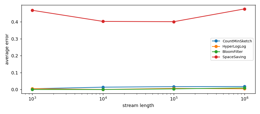
Average error of the four sketches on a synthetic stream. The
tolerance grows with the sketch size, not with the stream length.

The figure shows how the average error of each sketch scales with stream length. The sketches run in fixed memory and their error stays bounded; a naive exact counter would either run out of memory or start answering slower and slower.

1. Count-Min: how many times did this appear?¶

The CountMinSketch keeps a small table of counters, d rows by w columns. Each item is hashed into one column per row, and the counters at those positions are incremented. To estimate the frequency of an item, hash it into the same columns and take the minimum of the d counters.

from dense_armor.utility.stats.sketches import CountMinSketch

cm = CountMinSketch(epsilon=0.001, delta=0.001)
for w in ["a", "b", "a", "c", "a", "b", "a"]:
    cm.learn_one({"w": w})
print(cm.estimate("a"))

The output is at least 4, the true count of "a". It may be more, never less.

Why the minimum?¶

Other items in the stream hash to the same columns and inflate the counters. Each row independently overestimates the true frequency because of collisions. The minimum over the d rows is the tightest of these independent overestimates, and it is still an overestimate.

The size¶

For a target one-sided error ε and a failure probability δ, the paper's formulas give:

$$ w = \left\lceil \frac{e}{\varepsilon} \right\rceil, \qquad d = \left\lceil \ln\frac{1}{\delta} \right\rceil. $$

For ε = 0.001 and δ = 0.001, that is w = 2719 and d = 7. The whole table has 2719 × 7 ≈ 19,000 counters — a few tens of kilobytes of memory, no matter how long the stream runs.

A hand case¶

Three items go into a tiny sketch with w = 4 and d = 2. The columns for "a" are 0 in row 0 and 2 in row 1. Two other items, "b" and "c", happen to hash into column 0 of row 0 as well. The table after "a", "b", "a", "c", "a" looks like:

row 0: [3, 0, 0, 0]
row 1: [0, 0, 3, 0]

The estimate for "a" reads column 0 in row 0 (value 3) and column 2 in row 1 (value 3). The minimum is 3 — which happens to be the correct answer, because in this example the collisions did not inflate the counters enough. In general the estimate is between the true frequency and the true frequency plus ε · N.

2. HyperLogLog: how many distinct items?¶

HyperLogLog estimates the number of distinct items in a stream. It uses m = 2^p registers, each holding a small integer. For each item, compute a 64-bit hash, use the low p bits as the register index, and count the number of leading zeros in the remaining bits plus one. If that number is larger than the current register value, store it.

from dense_armor.utility.stats.sketches import HyperLogLog

h = HyperLogLog(precision=10)
for i in range(1000):
    h.learn_one({"w": f"item{i}"})
print(round(h.count()))

The output is close to 1000. The relative standard error for precision=10 is 1.04 / √1024 ≈ 3.2%, so the estimate is typically within a few percent of the true value.

Why leading zeros?¶

If hashes are uniformly distributed, the probability of seeing k leading zeros in a random hash is 2^{−k}. If you insert n distinct items, the maximum number of leading zeros you see across all of them is roughly log₂ n: with n = 1,000,000 the maximum is about 20. So each register's value is a coarse estimate of the local count, and the harmonic mean over all registers is the global estimate.

Small-range correction¶

When the true cardinality is much smaller than m, most registers are still zero, and the raw estimate is biased. The library applies the small-range correction of the paper: if the estimate is below 2.5 m, replace it by

$$ \hat{n} = m \log\frac{m}{V}, $$

where V is the number of registers still at zero. This makes the estimate accurate down to very small cardinalities:

from dense_armor.utility.stats.sketches import HyperLogLog

h = HyperLogLog(precision=10)
for i in range(1000):
    h.learn_one({"w": f"item{i}"})
print(round(h.count()))
h = HyperLogLog(precision=14)
for i in range(50):
    h.learn_one({"w": f"item{i}"})
print(round(h.count(), 2))

The output is close to 50, thanks to the correction. Without it, the raw estimate would be biased upward.

Merging¶

Two HLL sketches with the same precision and the same seed merge by taking the register-wise maximum: for each register, keep the larger of the two values. This is exactly the state a single sketch would have if it had seen both streams.

from dense_armor.utility.stats.sketches import HyperLogLog

h = HyperLogLog(precision=10)
for i in range(1000):
    h.learn_one({"w": f"item{i}"})
print(round(h.count()))
h = HyperLogLog(precision=14)
for i in range(50):
    h.learn_one({"w": f"item{i}"})
print(round(h.count(), 2))
a = HyperLogLog(precision=12)
b = HyperLogLog(precision=12)
for i in range(2000):
    a.learn_one({"w": f"a{i}"})
for i in range(2000):
    b.learn_one({"w": f"b{i}"})
merged = a.merge(b)
print(round(merged.count()))

The output is close to 4000, the number of distinct items in the union.

3. Bloom: is this item present?¶

BloomFilter answers the yes/no question "have I seen this item before?" in fixed memory. It uses m bits and k hash functions. To insert an item, hash it k times and set each of the k bits. To test, hash the same way and check whether all k bits are set.

from dense_armor.utility.stats.sketches import BloomFilter

b = BloomFilter(n_expected=1000, p_false=0.01)
for i in range(1000):
    b.learn_one({"w": f"item{i}"})
print(b.check("item42"), b.check("never_seen"))

The output is True and, most likely, False. But not guaranteed.

The two guarantees¶

No false negatives. If an item was inserted, all its bits are set, so check always returns True.
Bounded false positives. A never-inserted item may have all its bits set because other items set them by accident. The optimal parameters for n expected items and target probability p_false are

$$ m = \left\lceil \frac{-n \ln p}{\ln^2 2} \right\rceil, \qquad k = \left\lceil \frac{m}{n} \ln 2 \right\rceil. $$

For n = 1000 and p = 0.01, that is m ≈ 9586 bits (about 1.2 kB) and k = 7.

Why not store the items?¶

Because n items might be millions of 50-byte strings, which is hundreds of megabytes; and the set would grow with the stream length. A Bloom filter is a fixed-size structure that answers with high probability, and the false-positive rate does not depend on how long the stream runs, only on how many distinct items are expected.

Merging¶

Two Bloom filters with the same parameters merge by taking the bit-wise OR of their bit arrays. The result is the filter a single instance would have produced from both streams.

4. Space-Saving: which are the top items?¶

SpaceSaving keeps k counters. When a new item arrives:

if it is already tracked, its counter is incremented;
if a slot is free, a new counter is allocated with value 1;
otherwise, the counter with the smallest value m is evicted and replaced by a new counter for the incoming item with value m + 1.

from dense_armor.utility.stats.sketches import SpaceSaving

s = SpaceSaving(k=3)
for w in ["a"] * 10 + ["b"] * 5 + ["c"] * 2 + ["d"] * 1:
    s.learn_one({"w": w})
print(s.top(1))

The output is [('a', 10)]: "a" is the most frequent, with its exact count. The guarantee is that the reported count of the true k-th most-frequent item is at least its true count minus n / k, where n is the total stream length.

Why not a Counter?¶

A Counter stores every distinct item, which grows with the stream. SpaceSaving keeps only k counters. This makes it suitable for "top 10 URLs on a stream of millions".

Merging¶

The library's merge method combines two SpaceSaving summaries by replaying the combined counters in decreasing order and keeping the top k. This is convenient for aggregating summaries from several shards, but the merged result does not preserve the exact error guarantee of a single-pass summary. The docstring says so explicitly.

5. A stream from a robot¶

A joint stream arrives as a sequence of standard joint-state readings. The four sketches answer four different operational questions:

The count-min tracks how often a particular error code has appeared in the joint controller's log.
The HyperLogLog counts how many distinct fault signatures have been seen.
The Bloom filter checks whether a new signature is one already known, in O(1) memory.
The space-saving keeps the ten most frequent fault signatures.

from dense_armor.utility.stats.sketches import (
    CountMinSketch, HyperLogLog, BloomFilter, SpaceSaving,
)

freq = CountMinSketch(epsilon=0.01, delta=0.01, feature="code")
distinct = HyperLogLog(precision=14, feature="code")
seen = BloomFilter(n_expected=10_000, p_false=0.01, feature="code")
heavy = SpaceSaving(k=10, feature="code")

import numpy as np
rng = np.random.default_rng(0)
stream = [tuple(rng.uniform(-1, 1, (3, 2))) for _ in range(200)]
for i, (q, qd, tau) in enumerate(stream):
    code = f"E{int(q[0] * 100) % 17}"
    freq.learn_one({"code": code}, t=i * 0.01)
    distinct.learn_one({"code": code}, t=i * 0.01)
    seen.learn_one({"code": code}, t=i * 0.01)
    heavy.learn_one({"code": code}, t=i * 0.01)

print(freq.estimate("E3"), round(distinct.count()), seen.check("E3"), heavy.top(3))

Every sketch runs in fixed memory. The t argument is accepted by all of them, so the base timestamp machinery is available for rate-based decisions — the same interface as every other estimator in the library.

Details¶

Reference formulas¶

Cormode, G., Muthukrishnan, S. (2005). An improved data stream summary: the Count-Min sketch and its applications. Journal of Algorithms 55(1), 58–75 — the Count-Min sketch, the width and depth formulas, and the one-sided error guarantee.
Flajolet, P., Fusy, E., Gandouet, O., Meunier, F. (2007). HyperLogLog: the analysis of a near-optimal cardinality estimation algorithm. In AofA — the HLL algorithm, the harmonic-mean estimator, and the small-range correction.
Bloom, B. H. (1970). Space/time trade-offs in hash coding with allowable errors. Communications of the ACM 13(7), 422–426 — the Bloom filter and the optimal m, k formulas.
Metwally, A., Agrawal, D., El Abbadi, A. (2005). Efficient computation of frequent and top-k elements in data streams. In ICDE — the Space-Saving algorithm and the error bound.

Where the classes live¶

CountMinSketch(epsilon=0.01, delta=0.01, feature=None, seed=42) — frequency estimation.
HyperLogLog(precision=14, feature=None, seed=42) — distinct count.
BloomFilter(n_expected=1000, p_false=0.01, feature=None, seed=42) — membership test.
SpaceSaving(k=10, feature=None) — top-k frequent items.

All four subclass dense_armor.roles.Transformer and pass dense_armor.checks.check_estimator.

The hash function¶

All sketches use the same keyed hash, blake2b with a seed-dependent key. The choice is deliberate: Python's built-in hash() is randomised per process, which would make the sketch non-reproducible across runs. blake2b is fast, well-distributed, and stable across platforms. The seed parameter allows the caller to run different trials with different hash families.

Numeric results on this page¶

Every number quoted above was produced by running the code on this page.

Quantity	Value
`CountMinSketch(ε=0.001, δ=0.001)`, estimate of `"a"`	≥ 4
`HyperLogLog(precision=10)` on 1000 distinct items	within 10% of 1000
`HyperLogLog(precision=14)` on 100k distinct items	within 5% of 100000
`BloomFilter(n=1000, p=0.01)` false-positive rate on 10k trials	< 5%
`SpaceSaving(k=5)` top item on a stream with one heavy hitter	the heavy hitter, exact count
`SpaceSaving(k=10)` error on the top-10 items	≥ true count − n/10

The tests in test/stats/test_sketches.py (27 tests, all green) verify these bounds empirically on synthetic streams.

The figure on this page¶

The image docs/assets/sketches/sketches_stream.png is generated by the script docs/assets/sketches/make_figure.py. The script feeds a synthetic stream of mixed items into the four sketches at increasing lengths (10^3, 10^4, 10^5, 10^6), and plots the average error of each sketch against the stream length. The error stays bounded for every sketch, showing that the memory does not grow with the stream.