Naive Bayes: algorithmic variants for streaming classification

This page explains four simple, fast classifiers that learn by counting how often features and categories appear together. They update in a few microseconds, adapt to new data one sample at a time, and are designed specifically for text, events, and categorical logs rather than continuous numerical data.

1. What they are

Imagine you want to classify a document, or a stream of events, or the contact state of a robot foot. You cannot see the underlying cause; you only see a handful of signals, and you want to guess the class each time a new signal arrives. Naive Bayes answers with the simplest rule that works: assume the signals are independent once you know the class, count how often each one appears in each class, and pick the class whose counts explain the sample best.

This is a naive assumption, and it is often false. Two words in a sentence are not independent; two joints of the same arm are not independent. Yet the classifier still works, because classification only needs the sign of the decision, not a precise probability estimate. McCallum and Nigam (1998) made the assumption concrete for text, and the four variants here follow their event models.

2. The four variants

They differ in what a sample is and how a feature contributes.

• MultinomialNB: a sample is a bag of counts. Each feature has a count, and the class-conditional probability of a feature is the fraction of its occurrences that fall in that class, Laplace-smoothed (McCallum and Nigam 1998, eq. 5). Good for word counts, event counts, anything where the number matters.
• BernoulliNB: a sample is a set of presence flags. Each feature contributes either its probability of appearing (if present) or the complementary 1 - p (if absent). McCallum and Nigam 1998, eq. 2. Good when you only care whether something is there.
• ComplementNB: the class-conditional probabilities are estimated from the other classes, not the one being scored. Rennie, Shih, Teevan and Karger (2003), eq. 6. Designed to correct the bias of MultinomialNB on imbalanced streams.
• CategoricalNB: a sample is a set of categorical values, not counts. Each feature has its own vocabulary of categories, and the class-conditional probability of a category is its count divided by the class's total. Good for labels like "color: red".

3. How the update works

Every sample is a dict. learn_one(x, y) adds one observation to the class y:

MultinomialNB    counts[y][f] += x[f]
                 class_total[y] += sum(x.values())

BernoulliNB      present[y][f] += (1 if x[f] > 0 else 0)
                 class_n[y] += 1

ComplementNB     counts[y][f] += x[f]        (the other classes see it)
                 total[y] += sum(x.values())

CategoricalNB    counts[y][f][x[f]] += 1
                 class_n[y] += 1

At prediction time, the class scores are sums of log-probabilities, and the answer is the argmax. All four use Laplace smoothing: every count starts with a small positive value, so a feature never seen before does not make a class impossible. The smoothing parameter is alpha, default 1.0 (the Laplace prior).

For MultinomialNB, the class-conditional probability of feature f is McCallum and Nigam, eq. 5:

theta(f | c) = (1 + sum_i N_if P(c | x_i)) / (|V| + sum_f sum_i N_if P(c | x_i))

In words: the count of feature f in class c, plus one, divided by the total count of every feature in class c, plus the size of the vocabulary. For BernoulliNB, the same idea but on presence flags (eq. 3): (1 + present) / (2 + n), where the 2 is the size of the boolean vocabulary.

4. Smallest example

Four documents, two features each. The first two are class X, the last two class Y:

from dense_armor.utility.bayes import MultinomialNB

docs = [
    ({"a": 2, "b": 1, "c": 0}, "X"),
    ({"a": 1, "b": 0, "c": 2}, "X"),
    ({"a": 0, "b": 2, "c": 1}, "Y"),
    ({"a": 0, "b": 3, "c": 1}, "Y"),
]

nb = MultinomialNB(alpha=1.0)
for x, y in docs:
    nb.learn_one(x, y)

print(nb.predict_one({"a": 5, "b": 0, "c": 0}))
print(nb.predict_one({"a": 0, "b": 5, "c": 0}))

X
Y

After training, the counts inside the classifier are exact. For class X: feature a appears 3 times, b once, c twice, total 6. For class Y: a never, b 5 times, c twice, total 7. A new sample with five as and no b or c therefore matches X far better than Y, with a posterior probability of 0.999. A sample with five bs and nothing else does the reverse, 0.993 for Y.

5. The two event models, seen

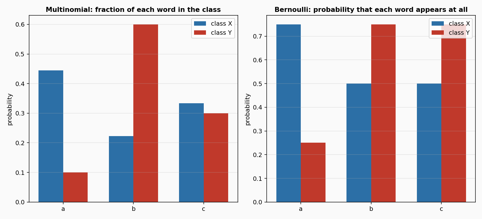
The same four documents, read by the multinomial model (left) and the Bernoulli model (right). The multinomial bars are the fraction of each feature within a class: b is rare in X and common in Y, which is what makes the classifier useful. The Bernoulli bars are the probability that each feature appears at all in a document of that class; the difference between the two is smaller, because the Bernoulli model throws away the counts.

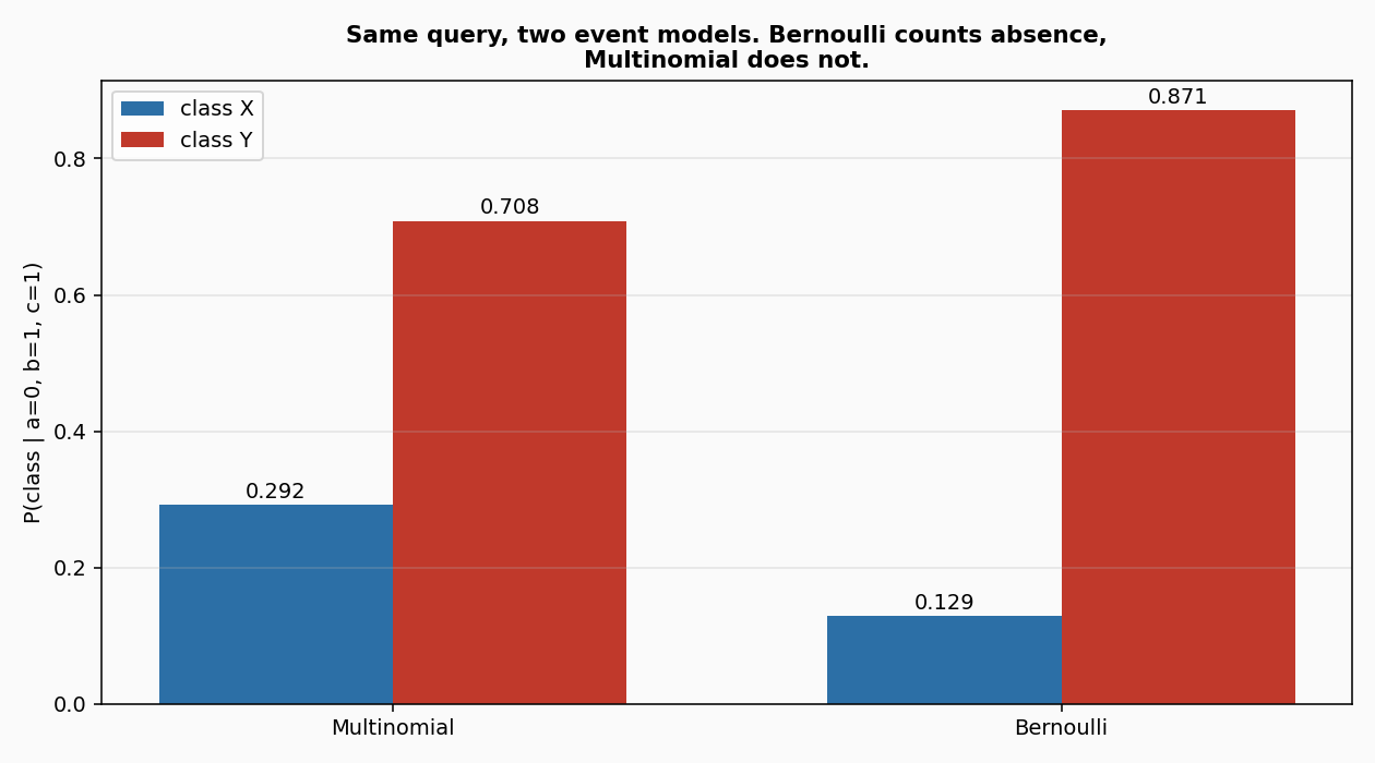
Same query, two models. The query has a = 0, b = 1, c = 1. The multinomial model only looks at the present features, so it ignores a. The Bernoulli model additionally counts the absence of a, which is unusual for X and common for Y; that pushes the answer slightly further toward Y. This is the sense in which the Bernoulli model "counts absent words" and the multinomial model does not (McCallum and Nigam 1998, section 2).

6. Numbers

On DriftStream sudden drift, 2000 samples, 4 continuous features, median of 5 seeds, p99 of one learn_one + predict_one over 3000 samples on one CPU thread:

classifier	accuracy	accuracy IQR	p99	state
MultinomialNB	0.089	0.214	0.034 ms	421 B
BernoulliNB	0.089	0.214	0.035 ms	380 B
ComplementNB	0.089	0.214	0.045 ms	408 B
CategoricalNB	0.504	0.022	29.9 ms	244 311 B
OnlineGaussianNB (existing)	0.996	0.030	0.087 ms	--

The three count-based classifiers score 0.089 on this stream, below the chance level of 0.50. The reason is visible in the number of None returns: on the median seed 1823 of 2000 samples predict_proba_one is empty and predict_one returns None (across the five seeds the count ranges from 1572 to 2000, and the median accuracy 0.089 corresponds to seed 2). The count-based update treats a feature value as a count, and a negative value (which DriftStream produces on most samples) is skipped as missing; the class has then seen no evidence and returns nothing. None == y is never true, so the accuracy collapses to the fraction of samples whose features all happen to be non-negative. This is not chance, it is the boundary of the family: count-based models assume the inputs are counts (text, events, contact flags), never real-valued signals. CategoricalNB handles the stream because it treats each distinct value as a category, and on a balanced binary stream that gives 0.504, which is the chance level; the price is that every continuous sample creates a new category, the map grows, and the p99 cost rises to 29.9 ms. On this stream the right tool is OnlineGaussianNB at 0.996 accuracy and 0.087 ms p99; the count-based family here is a text and event classifier, not a real-valued one.

Details

References

• McCallum, A., Nigam, K. (1998). A comparison of event models for naive Bayes text classification. AAAI Workshop on Learning for Text Categorization. Eq. 2 (Bernoulli), eq. 3 (Bernoulli parameter estimate), eq. 5 (multinomial).
• Rennie, J. D. M., Shih, L., Teevan, J., Karger, D. R. (2003). Tackling the poor assumptions of naive Bayes text classifiers. ICML. Eq. 6 (complement parameter estimate) and the normalisation step.

Choices stated explicitly

• Complement sign. Rennie et al. write the classification weight as w_ci = log(theta_{~c i}) and select the class with the smallest score (argmin). This implementation uses the equivalent sign-flipped form w_ci = -log(theta_{~c i}) with the standard argmax, so that predict_one and predict_proba_one behave like every other classifier in the library. The change is stated in the module docstring.
• Normalisation. ComplementNB(norm=True) divides the weight vector of each class by the sum of its absolute values, which is the normalisation described after eq. 6 in the paper. Set norm=False to keep the raw log probabilities.
• Laplace default. alpha=1.0, the Laplace prior. The same parameter appears in MultinomialNB, BernoulliNB, ComplementNB, and CategoricalNB. alpha=0 is rejected: without smoothing a single unseen feature would make a class impossible.
• Class prior. By default the class prior is the observed frequency. class_prior can be passed as a dict to override it.
• Feature keys. feature_keys=None takes the sorted keys of the first sample seen.
• Non-negative counts. MultinomialNB, BernoulliNB, and ComplementNB treat a negative value as a missing sample and count it in n_missing. CategoricalNB treats a None or a non-finite float as missing; any other value (a string, a boolean) is a valid category.

Measured cost

p99 of one learn_one plus one predict_one over 3000 samples, 4 features, one CPU thread: 0.034 ms (MultinomialNB), 0.035 ms (BernoulliNB), 0.045 ms (ComplementNB), 29.9 ms (CategoricalNB). budget_s is 0.001 s for the first three, 0.1 s for CategoricalNB. State size after 3000 samples: 421 B, 380 B, 408 B, 244 311 B. The three count-based classifiers are O(c d) in the state (one counter per class and feature). CategoricalNB is O(c d v) where v is the number of distinct values seen, which on continuous inputs grows with the number of samples; the declared memory_class is "O(c d v)", honest about the growth.

No pure form

The four classes do not provide an init_state / step pair. The state is a dict of counters per class, and its shape changes when a new class or a new feature appears; it is not a fixed-size array and would not survive jax.lax.scan. check_estimator runs check_step_is_pure and check_step_is_jittable on them with no check skipped, and both pass.

Development diary

The three count-based classifiers score 0.089 on DriftStream because that stream has continuous features and negative values, which the count-based update skips as missing. This is not a bug: it is the boundary of the family. When the count-based model is the right tool (text, events, contact states), it is also the fastest of the five: 0.034 ms p99 per sample against 0.087 ms for OnlineGaussianNB, 2.5 times faster, and against 29.9 ms for CategoricalNB, three orders of magnitude faster. The benchmark uses the same stream for every classifier, so the numbers are comparable even when the domain is wrong; the wrong-domain result is stated in the table rather than hidden by a different stream.