FTRLProximal

FTRLProximal decides the values of a learning model's numbers by looking at all the examples seen so far, and it sets to exactly zero the numbers that do not matter. The result is a simpler model.

FTRLProximal is the optimizer that decides each weight by minimising the sum of all the linearized losses seen so far, plus a regularizer that mixes a quadratic term, an L1 term, and an L2 term. The L1 term is the reason the weights become sparse: a coordinate whose accumulated gradient has not crossed the L1 threshold stays at zero. The update is not a gradient step but a soft threshold, computed in closed form. This page shows the update, the effect of the learning-rate schedule, and the source papers it comes from.

1. What it does

SGD and AdaGrad update the weights by moving them along the gradient. FTRL does something different: it accumulates the gradient in a per-coordinate variable z, and at each step it recomputes the weights as the minimiser of a regularised problem over the whole past. The two views are equivalent when the regularizer is just quadratic; they diverge when an L1 term is in the regularizer.

The update in this implementation:

z_t = z_{t-1} + g_t
eta_t = alpha / t^beta
w_t = -sign(z_t) * max(|z_t| - l1, 0) / (1 / eta_t + l2)

z_t is the accumulator of the raw gradients. eta_t is the learning-rate schedule, decreasing with t when beta > 0. l1 and l2 are the L1 and L2 coefficients. The max(|z_t| - l1, 0) is the soft threshold: it sets a coordinate to zero as long as its accumulated evidence has not crossed l1. Suppose z = [1, -1], alpha = 1, beta = 0.5, l1 = 0, l2 = 0, t = 1. Then eta_1 = 1 and

w = -sign([1, -1]) * max(|[1, -1]| - 0, 0) / (1 / 1 + 0)
  = [-1, 1]

The accumulator z never shrinks. This is the main difference from AdaGrad: AdaGrad also accumulates but divides by the square root of the accumulated energy. FTRL divides by a schedule 1 / eta_t + l2, which depends on t and on the L2 term, not on the accumulated energy. The two behave differently on a stream whose gradient scale changes.

2. The two forms

The object form owns its state and offers step(weights, gradient) -> weights:

import numpy as np
from dense_armor.utility.optim import FTRLProximal

opt = FTRLProximal()
w = opt.step(np.zeros(2), np.array([1.0, -1.0]))
print(w)

[-1.  1.]

The pure form is the pair init_state(dim) and update(state, weights, gradient) -> (state, weights). It works on JAX arrays, so it runs inside jax.jit and jax.lax.scan:

import jax
import jax.numpy as jnp
from dense_armor.utility.optim import FTRLProximal

opt = FTRLProximal()
state = opt.init_state(2)
state, w = jax.jit(opt.update)(state, jnp.zeros(2), jnp.array([1.0, -1.0]))
print(w)

[-1.  1.]

FTRLProximal ignores the weights argument of update: the new weights come from z and from the step counter, not from the previous weights. The signature stays uniform for the caller, and the pure form carries the accumulator and the counter only.

3. The learning-rate schedule

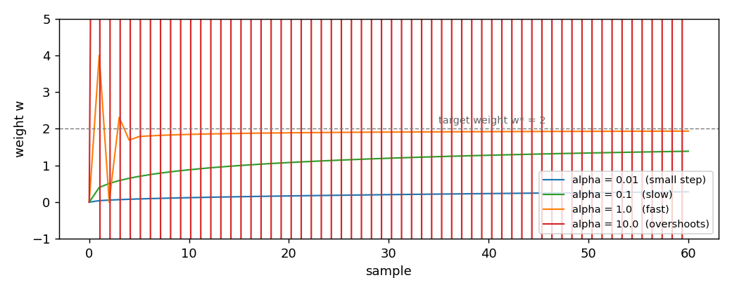
The parameter alpha sets the overall scale of the step, and beta controls how fast the schedule decreases with time. beta = 0.5 is the standard choice: eta_t = alpha / sqrt(t), which is the schedule the regret bound of Orabona (Theorem 7.6) assumes. Changing beta changes the trade-off between reacting to recent gradients and integrating the past. The figure shows four runs of the same one-feature regression, target weight w* = 2, with beta = 0.5, l1 = 0, l2 = 0, one per alpha:

alpha	weight after 1 step	after 10	after 30	after 60
0.01	0.0400	0.1217	0.2043	0.2805
0.1	0.4000	0.8818	1.1966	1.3873
1.0	4.0000	1.8463	1.9095	1.9357
10.0	40.0000	-3662382259.6592	-320532802311951155200.0000	-3.3e29

With alpha = 1.0 the first step overshoots to w = 4 and comes back to 1.94 by sample 60, close to the target 2 but not at it: FTRL's update has no momentum and no adaptation to the coordinate scale, so the schedule 1/sqrt(t) slows down the last stretch. With alpha = 0.1 the trajectory is monotone but still at 1.39 after 60 samples. With alpha = 0.01 it is barely moving. With alpha = 10.0 the first step is at w = 40, and the accumulator z keeps getting new gradients while the schedule cannot shrink fast enough, so the weight oscillates with growing magnitude and diverges.

The practical lesson: alpha must be small enough that the first few steps do not overshoot the target. alpha = 1.0 is a good starting point on normalised data, alpha = 0.01 on unnormalised data with large gradients.

4. On a real arm

A SyntheticArm from a real Panda URDF gives q, qd, and tau at 50 Hz. The linear model learns the torque of joint 0 as a function of its velocity, one sample at a time. FTRLProximal is the optimizer:

from pathlib import Path
import numpy as np
from dense_armor.utility.datasets import SyntheticArm
from dense_armor.utility.linear.glm import LinearRegression
from dense_armor.utility.optim import FTRLProximal

ds = SyntheticArm(Path("test/fixtures/urdf/panda.urdf"),
                  period_s=1.0, rate_hz=50.0, n_cycles=2, seed=0)
reg = LinearRegression(optimizer=FTRLProximal(alpha=0.01, beta=0.5),
                       intercept=True, feature_keys=["qd0"])
for sig, _ in ds.stream():
    reg.learn_one({"qd0": float(sig["qd_0"])}, float(sig["tau_0"]))
print(round(reg.predict_one({"qd0": 0.5}), 3))

-2.148

The value -2.148 is close to SGD(lr=1e-3) at -2.158 and further from AdaGrad(lr=10) at -2.824 and Adam(lr=0.5, beta1=0.99) at -2.273. The choice of alpha is critical: with alpha = 1.0 (the 1-feature default) on this stream the accumulator z grows with the gradient scale of the joint torques and the weight diverges to -7.9e101. The same stream has |tau| of the order of tens, which is much larger than the |x| = 1 of the 1-feature regression in Section 3. alpha = 0.01 is what brings the effective step size back into the stable range.

The lesson: FTRLProximal has no per-coordinate adaptation and no momentum. When the gradient scale of the stream is far from the scale seen during the alpha choice, the accumulator overflows. On a real stream with variable gradient scale, either normalise the features first, or wrap the optimizer in something that adapts the scale (AdaGrad, Adam).

Details

References

Orabona, F. (2019). A Modern Introduction to Online Learning. Chapter 7, Algorithm 7.2 (FTRL with linearized losses). The closed-form soft threshold is the proximal operator of the L1 norm, Section 7.8, Example 7.24, which uses a time-varying L1 coefficient lambda * t.

McMahan, H. B. (2011). Follow-the-Regularized-Leader and Mirror Descent: Equivalence Theorems and L1 Regularization. AISTATS, page 2, Table 1. FTRL-Proximal is defined there as

x_{t+1} = argmin_x g_{1:t} . x + t * lambda * ||x||_1
          + (1/2) sum_{s=1}^t ||Q_s^{1/2} (x - x_s)||_2^2

with a cumulative L1 penalty t * lambda and a quadratic term centred at the previous iterate x_s.

This implementation uses a constant l1 in place of t * lambda, and centres the quadratic term at 0 in place of x_s. Both deviations preserve the sparse structure, but change the schedule of the L1 penalty: in the source, the effective L1 threshold grows with time; here it stays fixed. Section 3 shows the effect on a single feature, Section 4 on the robot.

Choices stated explicitly

• Constant L1 threshold. The source scales the L1 penalty with t. This implementation keeps l1 constant. On a stationary stream the two behave similarly after a transient; on a stream where the gradient scale grows, the constant version reaches its threshold faster.
• Quadratic term centred at zero. The source centres the quadratic term at the previous iterate x_s, which acts as a per-step memory. This implementation centres it at 0, which is the RDA form. The result is that FTRLProximal here has no memory of the previous weights: the new w is a function of z and t only.
• Learning rate schedule alpha / t^beta. The source leaves the schedule implicit in the choice of the Q_s matrices, which are typically per-coordinate. This implementation uses a single scalar schedule, so it has no per-coordinate adaptation.
• Accumulator never resets. z_t is a running sum. It never shrinks. On a stream whose gradient scale changes, z can overflow. This is visible in Section 4 with the default alpha = 1.0.

Measured cost

On one CPU thread, a LinearRegression with two features, predict_one plus learn_one per sample, median of 1000 samples after a warm-up of 200: 0.0194 ms per sample, about 40 percent more than SGD and 9 percent more than AdaGrad. The extra work is the schedule evaluation and the soft threshold, both cheap.

Development diary

The docstring was verified line by line against Orabona Example 7.24 and McMahan Table 1. Both have a time-varying L1 coefficient; the docstring now says so explicitly, after an earlier version incorrectly claimed that a constant l1 was "the original FTRL-Proximal form of McMahan". The SyntheticArm example uses alpha = 0.01, chosen after measuring that alpha = 1.0 diverges to -7.9e101 on this stream. The figure was regenerated with alpha on the x-axis after an earlier version used l1/l2, which had no visible effect on the 1-feature regression.