Online metric learning: sequential Mahalanobis distance optimization

To find which past situations look like the current one, you need a way to measure the distance between them. Instead of assuming standard Euclidean formulas that get confused by noise, this tool learns a custom distance metric in real time from examples, so that situations that behave the same stay close together.

A robot arm picks objects. It has seen thousands of grasps: some worked, some did not. When a new situation arrives, the first thing any retrieval or imitation step needs to answer is "which past situations look like this one?"

"Look like" is a distance. The default answer is Euclidean distance on the raw feature vector. On real robot features it is often the wrong answer: joint angles wrap around, velocities matter more than positions for some tasks and less for others, and two situations can have very different coordinates and still be the same grasp. The distance has to be learned from data, not assumed.

MetricKNNClassifier learns that distance online, one triplet or pair at a time, while the robot works. It uses one of three algorithms ported from their papers:

• OASIS (Chechik et al. 2009) — bilinear similarity from triplets (anchor, similar, different).
• LEGO (Jain et al. 2008) — LogDet-regularized Mahalanobis matrix from pairs with a target distance.
• POLA (Shalev-Shwartz et al. 2004) — pseudo-metric from similar / dissimilar pairs, kept positive semi-definite.

1. The data

A stream of grasp features, one per attempt. Each sample is a 2-D vector: two joint torques at the moment of contact. Label: which grasp type succeeded.

import numpy as np
rng = np.random.default_rng(42)
grasps_a = rng.normal([1.0, 0.0], 0.1, (200, 2))
grasps_b = rng.normal([0.0, 1.0], 0.1, (200, 2))
X = np.vstack([grasps_a, grasps_b])
y = np.array(["A"] * 200 + ["B"] * 200)

Euclidean distance on this data works, because the clusters are far apart. On a real robot they are not.

2. Learn a distance from triplets: OASIS

OASIS takes three samples at a time: an anchor xa, a similar sample xp, and a different sample xn. It learns a matrix W such that the bilinear similarity

s(x, x') = xᵀ W x'

is higher for (xa, xp) than for (xa, xn) by at least a margin of 1.

The formula, symbol by symbol

For an anchor xa, a similar xp, a different xn, define the loss

ℓ = max(0, 1 − s(xa, xp) + s(xa, xn))

If ℓ > 0 (the constraint is violated), the update is a single rank-one step:

V = xa (xp − xn)ᵀ
τ = min(C, ℓ / ‖V‖²)
W ← W + τ V

C is the aggressiveness: how large a single step is allowed to be. V is the rank-one direction that increases similarity to xp and decreases similarity to xn simultaneously. The step size τ is the loss divided by the squared gradient magnitude, capped at C.

Hand case

Start W = I, C = 0.1, xa = (1, 0), xp = (1, 0.2), xn = (0.8, 0).

s(xa, xp) = xaᵀ W xp = 1
s(xa, xn) = xaᵀ W xn = 0.8
ℓ = max(0, 1 − 1 + 0.8) = 0.8
xp − xn = (0.2, 0.2)
V = [[0.2, 0.2], [0, 0]]
‖V‖² = 0.08
τ = min(0.1, 0.8 / 0.08) = min(0.1, 10) = 0.1
W ← I + 0.1 · [[0.2, 0.2], [0, 0]] = [[1.02, 0.02], [0, 1]]

The (0, 0) entry of W and the off-diagonal entry increased. The next time the same triplet arrives, s(xa, xp) is 1.02, s(xa, xn) is 0.816: the margin grew.

from dense_armor.utility.learn.metric_learning import OASIS

learner = OASIS(C=0.1)
learner.learn_triplet({"x0": 1.0, "x1": 0.0},
                      {"x0": 1.0, "x1": 0.2},
                      {"x0": 0.8, "x1": 0.0})

OASIS's learned W is not required to be symmetric. The distance used downstream is built from M = WᵀW, which is always positive semi-definite.

3. Learn from pairs with a target distance: LEGO

LEGO takes two samples and a target squared distance y. It updates a PSD matrix A toward that target using a LogDet-regularized gradient step.

The formula, symbol by symbol

For a pair (u, v) with squared-distance target y and vector z = u − v:

ŷ = zᵀ A z                    (current squared distance)
a = η y ŷ − 1
ȳ = (a + √(a² + 4η ŷ²)) / (2η ŷ)
A ← A − η (ȳ − y) (A z)(A z)ᵀ / (1 + η (ȳ − y) ŷ)

η is the learning rate; ȳ is the closed-form optimal post-update distance, derived in the paper (Section 2.1). Because A is updated through a LogDet-divergence step, it stays positive definite by construction: no separate projection needed.

Hand case

Start A = I, z = (1, 0), target y = 0.5, learning rate η = 0.1.

ŷ = 1
a = 0.1 · 0.5 · 1 − 1 = −0.95
ȳ = (−0.95 + √(0.9025 + 0.4)) / 0.2 = 0.9564
A z = (1, 0)
(A z)(A z)ᵀ = [[1, 0], [0, 0]]
A ← I − 0.1 · (0.9564 − 0.5) · [[1, 0], [0, 0]] / (1 + 0.1 · (0.9564 − 0.5) · 1)
  = I − 0.04364 · [[1, 0], [0, 0]]
  = [[0.9564, 0], [0, 1]]

A₀₀ moved from 1 to 0.9564 — toward the target 0.5, but only partway, because the LogDet regularizer resists large single steps. This is what makes LEGO's parameter updates stable without any tuning of a projection radius.

from dense_armor.utility.learn.metric_learning import LEGO

learner = LEGO(eta=0.1)
learner.learn_pair({"x0": 1.0, "x1": 0.0},
                   {"x0": 0.0, "x1": 0.0},
                   0.5)

LEGO needs a target squared distance per pair. LEGO.percentile_targets computes the 5th/95th percentiles of same-class / different-class distances, as in Section 4 of the paper.

4. Learn a pseudo-metric from similar/dissimilar pairs: POLA

POLA learns a pseudo-metric from a stream of pairs labelled y = +1 (similar) or y = −1 (different). It keeps a matrix A and a threshold b; a pair is predicted similar when the squared Mahalanobis distance d = zᵀ A z is below b.

The formula, symbol by symbol

For a pair with z = u − v and label y ∈ {+1, −1}:

d = zᵀ A z
ℓ = max(0, y (d − b) + 1)
α = ℓ / (1 + ‖z‖⁴)
A ← A − y α z zᵀ
b ← b + y α

Then A is projected back onto the PSD cone. If A still has a negative eigenvalue, it is removed (the paper shows only a single eigenvalue can go negative, so removing one rank-one direction is enough).

Hand case

Start A = I, b = 1, z = (1, 1), label y = +1.

d = [1, 1] · I · [1, 1]ᵀ = 2
ℓ = max(0, 1 · (2 − 1) + 1) = 2
‖z‖⁴ = (√2)⁴ = 4
α = 2 / (1 + 4) = 0.4
A ← I − 1 · 0.4 · [[1, 1], [1, 1]] = [[0.6, −0.4], [−0.4, 0.6]]
b ← 1 + 0.4 = 1.4

The eigenvalues of the new A are 0.2 and 1.0 — both positive, no projection needed. The pair was "different" (label +1 means similar, but the distance was above the threshold, so the pair was violating), and the update shrank A along the direction of z to make that direction's distance smaller next time.

from dense_armor.utility.learn.metric_learning import POLA

learner = POLA()
learner.learn_pair({"x0": 1.0, "x1": 0.0},
                   {"x0": 0.0, "x1": 0.0},
                   1)

5. The k-NN classifier that learns its metric

A metric learner does not fit the Classifier / Regressor / Transformer types of an existing online-learning library: it learns from two or three samples at a time and outputs a distance. MetricLearner is the base class; MetricKNNClassifier is a k-NN classifier that uses the base classes of an existing online-learning library that uses the learner as its distance and — with learn_metric=True, the default — trains it online inside learn_one. Each new sample is paired with random samples from the window: a triplet for OASIS, a similar / dissimilar pair for POLA, a pair with a target distance for LEGO.

import numpy as np
from dense_armor.utility.learn.metric_learning import MetricKNNClassifier, OASIS

rng = np.random.default_rng(0)
y = rng.integers(0, 2, 400)
X = np.c_[y + 0.3 * rng.standard_normal(400), rng.standard_normal(400)]
knn = MetricKNNClassifier(OASIS(C=0.1), n_neighbors=1, window_size=1000)
hits = 0
for x, t in zip(X, y):
    hits += knn.predict_one({"x0": x[0], "x1": x[1]}) == t
    knn.learn_one({"x0": x[0], "x1": x[1]}, t)
print(hits / len(y))

0.9375

Two classes that differ only in the first feature; the k-NN learns its similarity with OASIS while it classifies, and gets 93.75 % of the 400 samples right, each predicted before it is learned.

The same advantage on robot data: three robot states told apart by two joint features, plus three noisy features with a much larger range that dominate the plain Euclidean distance.

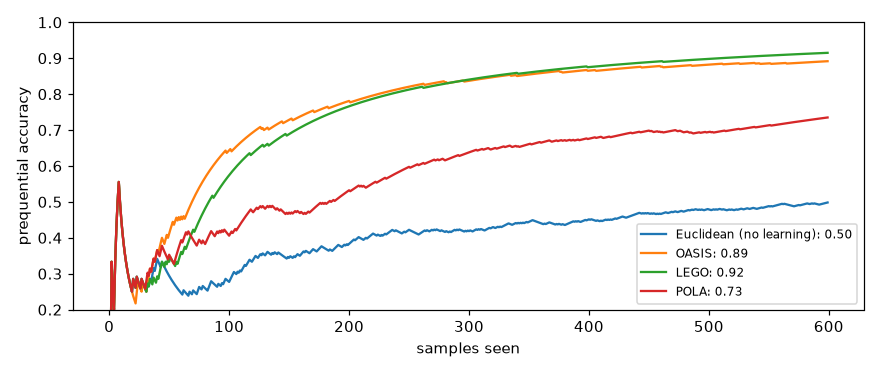
With the Euclidean distance the k-NN is right half of the time (0.50); learning the metric while classifying lifts it to 0.89 (OASIS), 0.92 (LEGO) and 0.74 (POLA) after 600 samples: the learned metric learns to ignore the noisy features. In the original paper OASIS already beat LEGO and the Euclidean metric on image retrieval (Chechik et al. 2009, Figure 2).

6. Results on streams from an existing online-learning library

progressive_val_score (predict, then learn), StandardScaler in front, k = 5, window_size=1000, metric learned online with the default parameters:

Stream	the other library's KNNClassifier (Euclidean)	OASIS	LEGO	POLA
Phishing (1,250 samples)	0.8823	0.8911 (+0.88)	0.8815 (−0.08)	0.8871 (+0.48)
ImageSegments (2,310 samples)	0.8705	0.9082 (+3.77)	0.9112 (+4.07)	0.9138 (+4.33)

On ImageSegments (7 classes, 18 features) all three learned metrics beat the Euclidean k-NN by about 4 points; on Phishing the gains are under one point and LEGO is level with the baseline.

API reference

metric_learning

Online metric learning: OASIS, LEGO and POLA, as estimators compatible with an existing online-learning library.

Needs the optional dependency: the streaming extra.

MetricLearner

Bases: Root

Root class for online metric learners.

A metric learner is trained from pairs or triplets and exposes a distance(x, x2) method. Unlike the Classifier, Regressor, and Transformer, it learns from relative information (two or three samples at a time) and does not predict labels or transform features directly.

Subclasses implement learn_triplet, learn_pair, and distance. Features are dicts; the first call fixes the feature order (sorted keys), and any feature not seen at that time counts as 0 in later calls.

learn_triplet

learn_triplet(x: dict, x_pos: dict, x_neg: dict) -> None

Update from a triplet (query, positive, negative).

Source code in dense_armor/utility/learn/metric_learning.py

def learn_triplet(self, x: dict, x_pos: dict, x_neg: dict) -> None:
    """Update from a triplet (query, positive, negative)."""
    raise NotImplementedError

learn_pair

learn_pair(x: dict, x2: dict, y) -> None

Update from a pair with a target (distance, or +/-1 label).

Source code in dense_armor/utility/learn/metric_learning.py

def learn_pair(self, x: dict, x2: dict, y) -> None:
    """Update from a pair with a target (distance, or +/-1 label)."""
    raise NotImplementedError

distance

distance(x: dict, x2: dict) -> float

Return the learned distance between two samples.

Source code in dense_armor/utility/learn/metric_learning.py

def distance(self, x: dict, x2: dict) -> float:
    """Return the learned distance between two samples."""
    raise NotImplementedError

OASIS

OASIS(C: float = 0.01)

Bases: MetricLearner

Online metric learning via passive-aggressive bilinear similarity.

Learns a bilinear similarity S(x, y) = x^T W y from triplets (query, positive, negative) such that S(x, x_pos) > S(x, x_neg) + 1. W is not constrained to be symmetric or positive semi-definite; the induced distance uses M = W^T W, which is always positive semi-definite.

Parameters

C Aggressiveness. The passive-aggressive step is min(C, loss / ‖V‖²). The paper recommends a small value; 0.01 to 0.1 works well in practice on standard benchmarks.

Examples

from dense_armor.utility.learn.metric_learning import OASIS oasis = OASIS(C=0.1) x = {"a": 1.0, "b": 0.0} x_pos = {"a": 0.9, "b": 0.1} x_neg = {"a": 0.1, "b": 0.9} _ = oasis.learn_triplet(x, x_pos, x_neg) oasis.distance(x, x_pos) < oasis.distance(x, x_neg) True

References

[^1]: Chechik, G., Sharma, V., Shalit, U. and Bengio, S., 2009. An online algorithm for large scale image similarity learning. In NIPS.

Source code in dense_armor/utility/learn/metric_learning.py

def __init__(self, C: float = 0.01):
    self.C = C
    self.W = None
    self._reset_features()

LEGO

LEGO(eta: float = 0.1)

Bases: MetricLearner

Online metric learning via LogDet regularization and exact gradient.

Learns a Mahalanobis matrix A from pairs (u, v) with a target squared distance y. Same-class pairs should have small targets, different-class pairs large ones; use percentile_targets to compute the 5th and 95th percentile of the pairwise distances of a training set, as in Section 4 of the paper.

Parameters

eta Learning rate of the LogDet gradient step. The paper uses 0.1.

Examples

from dense_armor.utility.learn.metric_learning import LEGO lego = LEGO(eta=0.1) u = {"a": 1.0, "b": 0.0} v = {"a": 0.0, "b": 1.0} d_before = lego.distance(u, v) _ = lego.learn_pair(u, v, 0.1) lego.distance(u, v) <= d_before True

References

[^1]: Jain, P., Kulis, B., Dhillon, I.S. and Grauman, K., 2008. Online metric learning and fast similarity search. In NIPS.

Source code in dense_armor/utility/learn/metric_learning.py

def __init__(self, eta: float = 0.1):
    self.eta = eta
    self.A = None
    self._reset_features()

percentile_targets staticmethod

percentile_targets(
    X, y, low: float = 5.0, high: float = 95.0
)

5th/95th percentile of same-class / different-class squared distances.

X is an array-like of shape (n, d), y an array-like of labels. Returns (near, far).

Source code in dense_armor/utility/learn/metric_learning.py

@staticmethod
def percentile_targets(X, y, low: float = 5.0, high: float = 95.0):
    """5th/95th percentile of same-class / different-class squared distances.

    X is an array-like of shape (n, d), y an array-like of labels.
    Returns (near, far).
    """
    X = np.asarray(X, dtype=float)
    y = np.asarray(y)
    D2 = np.sum((X[:, None, :] - X[None, :, :]) ** 2, axis=-1)
    same = y[:, None] == y[None, :]
    np.fill_diagonal(same, False)
    off = ~np.eye(len(X), dtype=bool)
    near = float(np.percentile(D2[same], low))
    far = float(np.percentile(D2[~same & off], high))
    return near, far

POLA

POLA(b_init: float = 1.0)

Bases: MetricLearner

Online pseudo-metric learning with PSD projection.

Learns (A, b) from labelled pairs (x, x2, y) with y = +1 for similar and y = -1 for dissimilar. After every update, A is projected onto the positive semi-definite cone and b onto [1, +inf).

Examples

from dense_armor.utility.learn.metric_learning import POLA pola = POLA() a = {"x": 0.0} b = {"x": 1.0} _ = pola.learn_pair(a, b, +1) _ = pola.learn_pair(a, b, -1) pola.b >= 1.0 True

References

[^1]: Shalev-Shwartz, S., Singer, Y. and Ng, A.Y., 2004. Online and batch learning of pseudo-metrics. In ICML.

Source code in dense_armor/utility/learn/metric_learning.py

def __init__(self, b_init: float = 1.0):
    self.b_init = b_init
    self.A = None
    self.b = b_init
    self._reset_features()

MetricKNNClassifier

MetricKNNClassifier(
    metric_learner: MetricLearner,
    n_neighbors: int = 5,
    window_size: int = 1000,
    learn_metric: bool = True,
    seed: int = 42,
    update_every: int = 1,
)

Bases: Classifier

K-nearest-neighbours classifier that learns its metric online.

Stores the last window_size samples and classifies a new sample by majority vote of its n_neighbors nearest neighbours under the metric learned by metric_learner. When learn_metric=True, every learn_one (every update_every steps) also feeds the metric learner with a pair or triplet built from the current window, so the metric adapts as the stream unfolds.

Parameters

metric_learner A MetricLearner (OASIS, LEGO or POLA). n_neighbors Number of nearest neighbours to vote. window_size Maximum number of stored samples (FIFO). learn_metric If True, learn_one also updates the metric learner. If False, the learner is only used as-is (frozen metric). seed Seed for the internal random.Random used to pick window samples. update_every Update the metric once every update_every calls to learn_one.

Examples

from dense_armor.utility.learn.metric_learning import MetricKNNClassifier, OASIS knn = MetricKNNClassifier(OASIS(C=1e6), n_neighbors=1, learn_metric=False) _ = knn.learn_one({"x": 1.0}, "A") _ = knn.learn_one({"x": 0.0}, "B") knn.predict_one({"x": 0.95}) 'A'

Source code in dense_armor/utility/learn/metric_learning.py

def __init__(self, metric_learner: MetricLearner, n_neighbors: int = 5,
             window_size: int = 1000, learn_metric: bool = True,
             seed: int = 42, update_every: int = 1):
    self.metric_learner = metric_learner
    self.n_neighbors = n_neighbors
    self.window_size = window_size
    self.learn_metric = learn_metric
    self.seed = seed
    self.update_every = update_every
    self._window = deque(maxlen=window_size)
    self.classes = set()
    self._rng = random.Random(seed)
    self._step = 0
    self._lego_targets_fixed = None

---

Details

OASIS (Chechik, Sharma, Shalit, Bengio, 2009). W is not symmetric; the distance uses M = WᵀW. The similarity is the bilinear form $S_W(p_i, p_j) = p_i^\top W p_j$ (eq. 2 of the paper) and the update is the passive-aggressive step $W \leftarrow W + \tau V$ with $\tau = \min(C,\; \ell_W / \lVert V\Vert^2)$ (eq. 5): "a gradient descent step with a step size τ that can be computed exactly", in the paper's words.

POLA (Shalev-Shwartz, Singer, Ng, 2004). The 1 + ‖z‖⁴ in the denominator is not a typo: the update is a projection of the pair $(A, b)$ onto a half-space, whose normal vector $\chi = (-y\, z z^\top,\; y)$ has squared norm $\lVert z z^\top\Vert_F^2 + 1 = \lVert z\Vert^4 + 1$; the + 1 comes from the threshold coordinate b. This gives $\alpha = \ell / (\lVert z\Vert^4 + 1)$ and the update of eq. 4 of the paper; a second projection onto the positive semi-definite cone (section 3.2) removes negative eigenvalues.

LEGO (Jain, Kulis, Dhillon, Grauman, 2008). The ȳ formula is equation (2.3) of the paper: the update (2.2) is the exact minimiser of the LogDet-regularised loss, written in closed form with the Sherman–Morrison formula; multiplying it on both sides by $z$ gives a quadratic equation in $\bar y$, whose positive root is (2.3). The LogDet step keeps A positive definite without projection: this is the difference between LEGO and POLA in the same online setting, and the reason LEGO has no separate "enforce PSD" step.

The three algorithms compared as kNN metrics on Iris, Wine, Digits and 20 newsgroups (including WᵀW against the symmetrized W) are in Dense-Evolution-Discovery, Online Metric Learning: OASIS, LEGO, POLA.

See also: Calibration — if the k-NN above is used with predict_proba_one, calibration turns its raw class frequencies into honest probabilities.