Drift detectors: sequential statistical architectures for concept drift isolation
This page explains how a system can notice slow, gradual changes in a robot's operational numbers before an outright mechanical failure occurs. By accumulating small deviations over time rather than looking at individual readings, these four tools can pinpoint exactly when a shift has happened, each trading off reaction delay against the rate of false alarms.
A robot that has been working fine for hours can start to behave differently without failing outright: a joint gets warmer and its torque creeps up, a new payload changes the load, a screw loosens and the vibration grows. The controller still works, but the numbers it reads are no longer the numbers it learned at the start. That is drift, and a robot that never notices it will slowly lose accuracy.
The problem is as old as statistical quality control. Shewhart's control chart (1931) watched a single sample against a fixed band and shouted as soon as one of them fell outside it. It worked for large, sudden faults, but it was blind to slow changes, because a small shift in the mean never makes a single sample look unusual. Page (1954) proposed the answer that is still the basis of every detector on this page: instead of judging each sample alone, accumulate the small deviations over time, so that a shift too small to notice in one reading still grows into a signal after enough of them.
A drift detector reads one number per sample and answers a single question:
has the behaviour changed? It must say so quickly, but it must not cry wolf:
a detector that fires on every small fluctuation is as useless as one that
stays silent. The four detectors on this page all use the same interface:
det.update(x) for one sample, and the flag det.drift_detected that becomes
True on the sample where the detector thinks something changed. Each one
trades delay for false alarms in a different way.
1. CUSUM with a fixed reference, even when the start is bad
The first detector, CUSUM, learns what "normal" looks like from the first samples it sees, then adds up how far each new sample is from it. When the sum grows past a threshold, it raises the flag. Missing readings at the start are skipped and counted, so a sensor that fails to deliver its first samples does not poison the reference.
Origins. Page, E. S. (1954), Continuous inspection schemes, Biometrika 41(1-2), 100-115. Page's idea was to keep a running sum of the distance between each sample and a reference, and to reset the sum whenever it would go negative. When the distributions before and after the change are known, Page's CUSUM is asymptotically optimal as the false-alarm rate goes to zero (Lorden 1971) and exactly optimal in Lorden's sense (Moustakides 1986), as recalled by Xie et al. (2021); here the reference is estimated from the first samples, so these results are a guide, not a guarantee.
import numpy as np
from dense_armor.utility.drift.detector import CUSUMDriftDetector

rng = np.random.default_rng(0)
x = [float("nan")] * 10 + list(rng.normal(0, 1, 300)) + list(rng.normal(3, 1, 300))
det = CUSUMDriftDetector(reference="fixed", radius=5, ref_mult=4)
first = next(i for i, v in enumerate(x) if det.update(v).drift_detected)
print(first, det.n_missing)
The step starts at index 310 (10 NaN + 300 normal samples). The detector
raises its first alarm at 315, five samples after the step, and reports ten
skipped readings in n_missing.
The CUSUM statistic is built from the distance between each sample and a reference, measured in robust standard deviations. If the sample sits close to the reference, the distance is small; if it drifts away, the distance grows and the accumulator climbs.
$$z_n = \frac{x_n - m}{s}, \qquad S_n = \max(0,\ S_{n-1} + z_n - k), \qquad \text{alarm when } S_n > h$$
Here $m$ and $s$ are the median and the robust scale of the first usable window, $k$ is the slack (how far a sample must deviate before it starts accumulating) and $h$ is the threshold on the sum. The defaults are $k = 0.5$ and $h = 20$.
The max(0, ...) is the reset: as long as a sample is close to the reference,
the accumulator falls back to zero and the detector forgets the small
fluctuations. Only a sustained deviation can push the sum high enough to
cross $h$.
For the full ARL derivation (average run length, how long before an alarm), the streaming API and the batch version, see CUSUM and ARL theory.
2. Page-Hinkley: the same idea, units do not matter
The second detector, Page-Hinkley, compares each sample with the running mean, measured in standard deviations. Because the comparison is in scale units, the same settings work whether the stream is a torque in N·m or a tiny squared error.
Origins. The name comes from Hinkley, D. V. (1971), Inference about the change-point from cumulative sum tests, Biometrika 58(3), 509-523, who turned Page's chart into an estimator of when the change happened. Dividing by the running standard deviation is this library's choice, so that the settings do not depend on the units of the stream.
import numpy as np
from dense_armor.utility.drift.page_hinkley import PageHinkley

rng = np.random.default_rng(0)
x = list(rng.normal(0, 1, 500)) + list(rng.normal(3, 1, 500))
for scale in (1.0, 1e-4):
    det = PageHinkley(delta=0.05, threshold=20.0)
    print(scale, next(i for i, v in enumerate(x) if det.update(scale * v).drift_detected))
The change starts at index 500. The detector fires at the same sample in both runs, once with the signal as it is and once with the signal multiplied by $10^{-4}$. The alarm index does not move, because the test uses standardized units.
The statistic is Page's cumulative sum: the samples are compared with the running mean, divided by the running standard deviation, and the accumulated deviation from the slack $\delta$ is compared with its own running minimum.
$$W_n = S_n - \min_{0 \le j \le n} S_j, \qquad S_n = \sum_{i \le n} \Big(\frac{x_i - \bar x_i}{\sigma_i} - \delta\Big)$$
Xie et al. (2021) write the same construction as equation 2, with the log-likelihood ratio in place of the standardized deviation.
Because both the reference mean and the reference scale move with the data, Page-Hinkley keeps working even when "normal" itself slowly drifts over a long recording. It is the same trade-off as CUSUM, with the reference sliding instead of fixed.
3. ADWIN: a window that cuts itself
ADWIN keeps the recent samples in a window and, at each step, tries every split of that window into an "older" and a "newer" part. If the two averages differ by more than chance alone allows, it drops the older part and reports a change.
Origins. Bifet, A., Gavaldà, R. (2007), Learning from time-changing data with adaptive windowing, Proceedings of the 2007 SIAM International Conference on Data Mining (SDM), 443-448. Bifet and Gavaldà were working on streaming classifiers that had to forget old data at the right moment: a fixed window is either too short (noisy) or too long (slow), and no single choice works for every stream. Their idea was to let the window choose its own length, by looking for a cut where the two halves disagree.
import numpy as np
from dense_armor.utility.drift.adwin import ADWIN

rng = np.random.default_rng(0)
x = list(rng.normal(0, 1, 300)) + list(rng.normal(4, 1, 300))
det = ADWIN(delta=0.002, max_window=100)
first = next(i for i, v in enumerate(x) if det.update(v).drift_detected)
print(first, len(det._window))
The change starts at index 300. The detector fires at 339 and, after the cut, keeps 40 samples in the window.
The threshold that decides whether the two averages are "too different" comes from Hoeffding's inequality. For two sub-windows of sizes $n_0$ and $n_1$, with values that lie in a range $R$, the probability that their sample averages differ by more than $\varepsilon$ by chance is at most
$$P\big(|\hat\mu_0 - \hat\mu_1| \ge \varepsilon\big) \le 2\,e^{-2m\varepsilon^2/R^2}, \quad m = \frac{n_0 n_1}{n_0 + n_1}, \qquad \varepsilon_\text{cut} = R\sqrt{\frac{\ln(2n/\delta)}{2m}}$$
where $m$ is half the harmonic mean of the two sub-window sizes. Solving for $\varepsilon$ at a total confidence level $\delta$, with a union bound over the $n$ possible cuts, gives $\varepsilon_\text{cut}$. $R$ is measured online from the range of the values currently in the window, so the detector does not depend on the units of the stream.
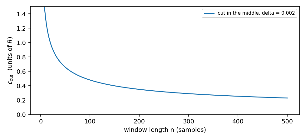
This bound is cautious on short windows: $\varepsilon_\text{cut}$ grows as the window gets shorter, because each side of the cut holds fewer samples and $m$ is small. With 100 samples in the window, ADWIN needs a step of about 4 standard deviations to fire; a 3σ step goes unnoticed.
One change can be flagged on several consecutive updates. ADWIN drops the oldest part of its window while
some cut passes the test; a change that has only just started leaves part of the old regime in the window,
and the test passes again a few updates later, once more of the new regime has arrived. On a step of 3
standard deviations, 500 samples into a stream, the first flag comes a few dozen samples after the step and
the burst ends within 100 samples (test/drift/test_adwin_alarms.py). Act on the first flag of a burst, or
start a new detector after it, to get one event per change.
The robot-stream table of section 5 uses this version of ADWIN.
4. KSWIN: compare the shapes, one alarm per change
KSWIN compares the newest 30 samples with 30 samples drawn at random from the older part of the window, using the Kolmogorov–Smirnov test. The test measures how far apart the two cumulative histograms are: a small distance means the two groups look alike, a large distance means they do not. After an alarm, the detector keeps only the newest samples, so a single change produces a single alarm.
Origins. Raab, C., Heusinger, M., Schleif, F.-M. (2020), Reactive soft prototype computing for concept drift streams, Neurocomputing 416, 340-351, arXiv:2007.05432. The authors were working on learning systems that keep a set of representative prototypes instead of a full model, and they needed to know when the prototypes had become stale. The Kolmogorov–Smirnov test is a classical two-sample test, free of distributional assumptions, so it fits a stream where the shape can change and not only the mean.
import numpy as np
from dense_armor.utility.drift.kswin import KSWIN

rng = np.random.default_rng(14)
x = list(rng.normal(0, 1, 400)) + list(rng.normal(2.5, 1, 400))
det = KSWIN(seed=0)
alarms = [i for i, v in enumerate(x) if det.update(v).drift_detected]
print(alarms)
The change starts at index 400, and the detector produces exactly one alarm, at 414. The default parameters come from Raab et al. (2020): a window of 300 samples, a sample of 30, and a significance level $\alpha = 10^{-4}$.
The reset after an alarm is not in the paper. Without it, KSWIN would keep firing on the same change for as long as the old and the new samples sit in the window together; with it, the detector answers once and waits for the next one.
5. The four side by side on a robot stream
The last test runs all four detectors on the CASPER dataset: a UR3e arm
sampled at 20 Hz, with a labelled change somewhere in the recording. The
signal used here is the squared shift residual of joint 5, averaged over 76 s
with a causal trailing mean; it is the same series the original CASPER
benchmark uses. The four detectors are run with their default settings,
untouched, through evaluate_events.
| detector | delay (s) | missed | false alarms / h |
|---|---|---|---|
| Page-Hinkley | 3.9 | 0 | 1041 |
| KSWIN | 7.8 | 0 | 217 |
| CUSUM (fixed reference) | 17.2 | 0 | 1188 |
| ADWIN | 17.7 | 0 | 1.4 |
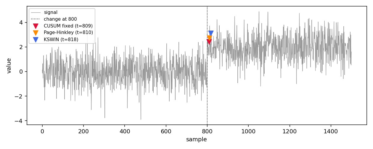
The figure above is a synthetic illustration of the same behaviour on a clean step: each marker is the first alarm of one detector, and the change is the dotted line. ADWIN has no marker: on a 2σ step with a window of 100 samples its bound is never crossed, as section 3 explains.
All four catch the change, none of them misses it. The false alarms are
counted over the whole recording. For the CUSUM they all come after the
labelled event — zero before the change — because a fixed reference keeps
firing while the level stays away from it. The CUSUM row matches the original
benchmark function run_cusum exactly: 17.2 s of delay, zero false alarms
before the change.
Faster is not automatically better. Page-Hinkley is the quickest to react, and also the one that fires the most on normal data; KSWIN takes about twice as long and produces five times fewer false alarms. CUSUM fixed is the slowest here and produces the most false alarms per hour, because once the level has moved, the fixed reference is permanently wrong and the detector keeps re-arming on every fluctuation. ADWIN is as slow as the fixed CUSUM, 17.7 s, and produces about one false alarm per hour, two orders of magnitude fewer than the others; its cost is the delay.
The CASPER dataset is not committed to this repository: benchmarks/casper_benchmark.py
expects it under a Kaggle path (industrial-robotic-arm-anomaly-detection), so the
numbers above are from the run where the dataset was present.
The right choice depends on the cost of a missed change against the cost of a spurious alarm. For a robot, a false alarm may mean stopping the line for inspection; a missed change may mean a worn joint that keeps degrading for another shift. Both costs are real, and only the application knows which one is worse.
API reference
page_hinkley 
Page-Hinkley test for a change in the mean of a scalar stream.
Page, E. S. (1954). Continuous inspection schemes. Biometrika 41(1-2), 100-115. The formulation used here is the log-likelihood-ratio CUSUM written down in Xie, Zou, Xie, Veeravalli (2021), "Sequential (Quickest) Change Detection: Classical Results and New Directions", Section II-C2: the log-likelihood ratio l(X) is accumulated and compared with its running minimum (eq. 2),
W_n = S_n - min_{0 <= k <= n} S_k, S_n = sum_{k=1}^{n} l(X_k),
and the detector alarms when W_n exceeds a threshold b (eq. 3, the maximum-likelihood form). With a Gaussian reference of unit variance the log-likelihood ratio reduces to (x - mu_ref) / sigma_ref - delta, where mu_ref is the running mean, sigma_ref the running standard deviation of the stream, and delta is the slack in scale units. Working in scale units makes delta and threshold independent of the stream units, so the same parameters detect the same change on x and on 1e-4 * x.
PageHinkley 
PageHinkley(
    delta: float = 0.005,
    threshold: float = 50.0,
    two_sided: bool = True,
    warmup: int = 30,
)
Bases: DriftDetector
Page-Hinkley test for a change in the mean of a scalar stream.
Parameters:
| Name | Type | Description | Default |
|---|---|---|---|
delta
|
float
|
reference slack, in scale units (multiples of the
running standard deviation). Classical choice: half the
shift size worth detecting. Default |
0.005
|
threshold
|
float
|
alarm threshold on the accumulated deviation from
its running minimum, in scale units. Default |
50.0
|
two_sided
|
bool
|
if |
True
|
warmup
|
int
|
number of samples skipped before the first check.
Default |
30
|
Examples:
>>> from dense_armor.utility.drift.page_hinkley import PageHinkley
>>> import numpy as np
>>> rng = np.random.default_rng(0)
>>> det = PageHinkley(delta=0.05, threshold=20.0)
>>> stream = list(rng.normal(0, 1, 500)) + list(rng.normal(2, 1, 500))
>>> for i, x in enumerate(stream):
...     _ = det.update(x)
...     if det.drift_detected:
...         print(i)
...         break
508
Source code in dense_armor/utility/drift/page_hinkley.py
adwin 
ADWIN drift detector (Bifet & Gavalda 2006).
Two algorithms share this name. The first one (Section 3.2 of the
paper) stores the window as an explicit list of samples and tests
every cut; the cost of update is O(W) with W the window size.
The second one (Section 3.3 of the paper, ADWIN2) stores the window
as an exponential histogram of buckets: level i holds buckets
that pack 2**i samples, each level keeps at most max_buckets
buckets, and when a level overflows its two oldest buckets are
merged into one at the level above. The number of buckets is
O(log W), so update costs O(log W) worst case and O(1)
amortised.
The cut threshold. For a partition of the window into a historical
part W0 (with n0 samples, mean mu0) and a recent part
W1 (with n1 samples, mean mu1), with m = n0 n1 /
(n0 + n1) the harmonic-mean-like factor, R the observed range
of the window, and delta' = delta / ln(n) the multiple-
hypothesis correction of Section 3.2 ("only O(log n) subwindows are
checked, which justifies using delta' = delta / ln(n)"), the window
is dropped when
|mu0 - mu1| > R sqrt( ln(4/delta') / (2 m) ).
Both sides carry the units of the data, so the detector is scale- invariant.
One change can be flagged on several consecutive updates. At each update the oldest buckets are dropped while some cut passes the test (Algorithm 1 of the paper); a change that has only just started leaves part of the old regime in the window, and as more samples of the new regime arrive the test passes again a few updates later. Act on the first flag of a burst, or start a new detector after it, if one event per change is wanted. Before this version the detector flagged a change once, later.
Memory: O(max_buckets * log W).
ADWIN 
Bases: DriftDetector
Adaptive Windowing drift detector.
Parameters:
| Name | Type | Description | Default |
|---|---|---|---|
delta
|
float
|
confidence parameter, in |
0.002
|
max_window
|
int
|
maximum window size before the oldest samples start
being dropped. Default |
200
|
min_sub
|
int
|
minimum sub-window size considered during the cut
scan. Default |
2
|
max_buckets
|
int
|
maximum number of buckets kept per level before the
two oldest are merged into one at the level above.
Default |
5
|
Raises:
| Type | Description |
|---|---|
ValueError
|
if |
Examples:
>>> from dense_armor.utility.drift.adwin import ADWIN
>>> import numpy as np
>>> rng = np.random.default_rng(0)
>>> det = ADWIN(delta=0.002, max_window=100)
>>> stream = list(rng.normal(0, 1, 300)) + list(rng.normal(4, 1, 300))
>>> for i, x in enumerate(stream):
...     _ = det.update(x)
...     if det.drift_detected:
...         print(i)
...         break
329
Source code in dense_armor/utility/drift/adwin.py
kswin 
KSWIN drift detector (Raab, Heusinger, Schleif 2020).
KSWIN keeps a sliding window of size window_size. The most recent
stat_size samples are the new sample; a second sample of the same
size is drawn at random from the older part of the window. The two are
compared with a two-sample Kolmogorov-Smirnov test; a drift is flagged
when the p-value falls below alpha. The random draw is seeded so a
run is reproducible.
The paper does not specify what to do with the window after an alarm.
This implementation keeps only the last stat_size samples, so a
single change produces a single alarm: the window has to refill to
window_size before the KS test runs again, and the refill uses
post-change samples only.
KSWIN 
KSWIN(
    alpha: float = 0.0001,
    window_size: int = 300,
    stat_size: int = 30,
    seed: int | None = None,
)
Bases: DriftDetector
Kolmogorov-Smirnov Windowing drift detector.
Parameters:
| Name | Type | Description | Default |
|---|---|---|---|
alpha
|
float
|
significance level of the two-sample KS test. Default
|
0.0001
|
window_size
|
int
|
total sliding window length. Default |
300
|
stat_size
|
int
|
size of each of the two samples compared by KS.
Default |
30
|
seed
|
int | None
|
seed of the random generator used to draw the reference
sample. Default |
None
|
Raises:
| Type | Description |
|---|---|
ValueError
|
if |
Source code in dense_armor/utility/drift/kswin.py
detector 
CUSUM drift detector for the streaming interface.
CUSUMDriftDetector 
CUSUMDriftDetector(
    radius: int = 10,
    ref_mult: int = 3,
    k: float = 0.5,
    h: float = 20.0,
    two_sided: bool = True,
    eps: float = 1e-09,
    reference: str = "adaptive",
)
Bases: DriftDetector
CUSUM drift detector matching the batch cusum_detector behaviour.
Parameters
radius, ref_mult
Causal window span = radius * ref_mult, same convention as
cusum_detector.
k
CUSUM slack, in robust-sigma units.
h
Decision threshold, in accumulated robust-sigma units.
two_sided
If True, both upward and downward shifts are monitored. If False,
only upward shifts are monitored.
eps
Degenerate-scale guard, same convention as cusum_detector.
reference
"adaptive" recomputes median and scale from a sliding causal
window every step, matching cusum_detector(reference="adaptive").
The reference drifts with the data, so a sustained shift is
caught at its leading edge, then stops accumulating once the
window catches up. The detection floor for a sustained step is
roughly 2.2 robust sigmas at h=20.
"fixed" computes median and scale once from the first span
usable (finite, non-flat) values and never updates, matching
cusum_detector(reference="fixed") and Page's original scheme.
Non-finite samples do not count towards span; the fixed buffer
keeps only the last span finite values, so a long flat start
does not make the buffer grow without bound, and the reference
is retried on every new sample until a usable one is found.
Examples
from dense_armor.utility.drift.detector import CUSUMDriftDetector import numpy as np det = CUSUMDriftDetector(reference="fixed") rng = np.random.default_rng(0) stream = list(rng.normal(0, 1, 500)) + list(rng.normal(1, 1, 500)) for i, x in enumerate(stream): ... _ = det.update(x) ... if det.drift_detected: ... print(i) ... break 516
Source code in dense_armor/utility/drift/detector.py
Details
- CUSUM
reference="fixed": before this version a stream that started with missing or flat readings left the detector without a usable reference, and silent forever. Now non-finite samples do not count towards the reference span; the reference is retried on a sliding window of the lastspanfinite values until its robust scale is usable, so a NaN or flat start no longer leaves the detector silent. - ADWIN: the original paper (Bifet and Gavaldà 2007) is not on arXiv; the bound above is derived here from Hoeffding's inequality and a union bound over the cuts. Memory O(W) (the whole window is kept), each update O(W). The paper's original implementation uses an exponential histogram that brings both to O(log W); the O(W) version is a deliberate simplification for streams of a few hundred samples per window.
- KSWIN: the paper does not say what to do with the window after an alarm;
keeping the newest
stat_sizesamples gives one alarm per change. - Benchmark: delays at 20 Hz; the table uses the trailing mean of e² over
2T = 1520 samples (76 s), the series the original CASPER benchmark uses;
joint 5. The synthetic figure in section 5 is generated by
docs/assets/drift/make_figure.pyfrom the library itself, on a clean Gaussian step for clarity. - Sources:
- Shewhart, W. A. (1931). Economic Control of Quality of Manufactured Product. Van Nostrand. The control chart.
- Page, E. S. (1954). Continuous inspection schemes. Biometrika 41(1-2), 100-115. The CUSUM.
- Hinkley, D. V. (1971). Inference about the change-point from cumulative sum tests. Biometrika 58(3), 509-523. The Page-Hinkley form.
- Lorden, G. (1971). Procedures for reacting to a change in distribution. Annals of Mathematical Statistics 42(6), 1897-1908. Asymptotic optimality of CUSUM.
- Moustakides, G. V. (1986). Optimal stopping times for detecting changes in distributions. Annals of Statistics 14(4), 1379-1387. Exact optimality of CUSUM.
- Bifet, A., Gavaldà, R. (2007). Learning from time-changing data with adaptive windowing. In Proceedings of the 2007 SIAM International Conference on Data Mining. ADWIN.
- Lu, J., Liu, A., Dong, F., Gu, F., Gama, J., Zhang, G. (2018). Learning under concept drift: a review. arXiv:2004.05785. ADWIN and Page-Hinkley described in one place.
- Raab, C., Heusinger, M., Schleif, F.-M. (2020). Reactive soft prototype computing for concept drift streams. Neurocomputing 416, 340-351, arXiv:2007.05432. KSWIN.
- Xie, L., Zou, S., Xie, Y., Veeravalli, V. V. (2021). Sequential (quickest) change detection: classical results and new directions. arXiv:2104.04186. The general CUSUM/Page/Shewhart framework.
- Kayan, H., et al. (2023). CASPER: a real-world dataset for anomaly detection in a robot arm. In IEEE PerCom Workshops. The robot benchmark.