OnlineNewtonStep

OnlineNewtonStep decides how much to change a learning model's numbers after each example. Unlike the simple rules, it also takes into account how sharply the error curves.

OnlineNewtonStep is the only second-order optimizer in the package. It keeps a running approximation of the Hessian of the loss, and it uses the inverse of that approximation as a preconditioner. On losses that are exp-concave, the method has a logarithmic regret bound in the number of samples, better than the square-root bound of the first-order methods on the same class. On a generic convex loss there is no such guarantee. This page shows the update, the role of the step-size parameter, and the class of losses where the method is meant to be used.

1. What it does

SGD, AdaGrad, and Adam move the weights along the gradient, scaled by a learning rate or by an accumulator. OnlineNewtonStep moves them along the gradient, scaled by the inverse of a running approximation of the Hessian. The approximation is the outer product of the gradients seen so far:

A_t = A_{t-1} + g_t g_t^T
w_{t+1} = w_t - (1 / gamma) A_t^{-1} g_t

A_t is the running Hessian approximation, g_t is the gradient on the current sample, gamma is a positive scalar that sets the overall step size. A_0 = eps * I, so A_0^{-1} = I / eps. The inverse A_t^{-1} is kept in the state and updated with the Sherman-Morrison formula, so no linear solve is needed. Suppose w = [0, 0], g = [1, 0], gamma = 1, eps = 1. Then

A_0 = I
A_1 = I + [1, 0] [1, 0]^T = [[2, 0], [0, 1]]
A_1^{-1} = [[0.5, 0], [0, 1]]
w_new = [0, 0] - [0.5, 0] / 1
      = [-0.5, 0]

The effect: the coordinate that has been excited (the first one, with g = 1) moves less than it would with SGD. The second coordinate, never excited, moves by zero. This is the Newton-style behaviour: the method takes large steps in directions that have not been explored and small steps in directions that have.

2. The two forms

The object form owns its state and offers step(weights, gradient) -> weights:

import numpy as np
from dense_armor.utility.optim import OnlineNewtonStep

opt = OnlineNewtonStep(gamma=1.0, eps=1.0)
w = opt.step(np.zeros(2), np.array([1.0, 0.0]))
print(w)

[-0.5  0. ]

The pure form is the pair init_state(dim) and update(state, weights, gradient) -> (state, weights). It works on JAX arrays, so it runs inside jax.jit and jax.lax.scan:

import jax
import jax.numpy as jnp
from dense_armor.utility.optim import OnlineNewtonStep

opt = OnlineNewtonStep(gamma=1.0, eps=1.0)
state = opt.init_state(2)
state, w = jax.jit(opt.update)(state, jnp.zeros(2), jnp.array([1.0, 0.0]))
print(w)

[-0.5  0. ]

OnlineNewtonStep keeps a matrix in the state, one row and one column per feature. On a problem with many features this is the most expensive state of the five optimizers in the package. The two forms give the same weights step by step.

3. The step-size parameter

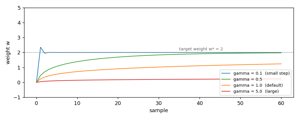
The parameter gamma divides the Newton-like step A_t^{-1} g_t. In the source paper, gamma is not free: it is fixed to gamma = (1/2) min(1 / (4 G D), alpha), where G is the maximum gradient norm, D is the diameter of the feasible set, and alpha is the exp-concavity constant of the losses. Here gamma is a free parameter with default 1.0. The figure shows four runs of the same one-feature regression, target weight w* = 2, one per gamma:

gamma	weight after 1 step	after 10	after 30	after 60
0.1	2.3529	2.0000	2.0000	2.0000
0.5	0.4706	1.3873	1.8360	1.9745
1.0	0.2353	0.7201	1.0248	1.2386
5.0	0.0471	0.1426	0.1976	0.2338

With gamma = 0.1 the method reaches the target in ten samples, faster than any first-order method in the package on the same problem. This is the second-order acceleration: the Hessian approximation grows with the number of samples, so the effective step size shrinks, and the weight settles on the target without oscillation. With gamma = 5.0 the effective step is five times smaller at every sample, and the weight is still far from the target after sixty samples.

The lesson: gamma is not a learning rate in the usual sense. It is a constant that multiplies the inverse Hessian. On a well-conditioned problem a small gamma is fast; on an ill-conditioned problem the same gamma can overshoot. Unlike the first-order methods, OnlineNewtonStep has no single "safe" default: the value that works on one problem may be off by a factor of ten on another.

4. On a real arm

A SyntheticArm from a real Panda URDF gives q, qd, and tau at 50 Hz. The linear model learns the torque of joint 0 as a function of its velocity, one sample at a time. OnlineNewtonStep is the optimizer:

from pathlib import Path
import numpy as np
from dense_armor.utility.datasets import SyntheticArm
from dense_armor.utility.linear.glm import LinearRegression
from dense_armor.utility.optim import OnlineNewtonStep

ds = SyntheticArm(Path("test/fixtures/urdf/panda.urdf"),
                  period_s=1.0, rate_hz=50.0, n_cycles=2, seed=0)
reg = LinearRegression(optimizer=OnlineNewtonStep(gamma=0.1, eps=1.0),
                       intercept=True, feature_keys=["qd0"])
for sig, _ in ds.stream():
    reg.learn_one({"qd0": float(sig["qd_0"])}, float(sig["tau_0"]))
print(round(reg.predict_one({"qd0": 0.5}), 3))

1.758

The value 1.758 is not close to the -2.158 of SGD(lr=1e-3), the -2.824 of AdaGrad(lr=10), the -2.273 of Adam(lr=0.5, beta1=0.99), or the -2.148 of FTRLProximal(alpha=0.01). It is also not zero, which means the model has learned something from the stream, but the sign is wrong relative to the true torque. This is the expected behaviour, not a bug.

The reason is the class of losses. OnlineNewtonStep has a logarithmic regret bound only on alpha-exp-concave losses, i.e. losses whose exponential exp(-alpha f) is concave. The squared loss of the joint-torque regression is not exp-concave on the whole real line: on unbounded domains its second derivative is constant, not bounded below by the gradient outer product. Without exp-concavity, the Newton-like step A_t^{-1} g_t is no longer guaranteed to reduce the loss, and the method can converge to a value different from the true minimum of the regression.

The lesson: OnlineNewtonStep is not a drop-in replacement for SGD. Use it when the loss is known to be exp-concave and the domain is bounded. On a generic regression task the first-order methods are the safer choice.

Details

References

Hazan, E., Agarwal, A., Kale, S. (2007). Logarithmic regret algorithms for online convex optimization. Machine Learning 69. In the manuscript of 20 November 2008 (log-regret.pdf) the algorithm is "Figure 3: The Online Newton Step algorithm", page 10; the journal version may number it differently. The update

A_t = A_{t-1} + g_t g_t^T
w_{t+1} = w_t - (1/gamma) A_t^{-1} g_t

follows Figure 3; the projection step is applied when D is given. Theorem 2, page 11, gives the regret bound

Regret_T <= 5 ((1/alpha) + G D) n log T

under the assumptions that the losses are alpha-exp-concave, that the gradients are bounded by G, and that the feasible set has diameter D.

Orabona, F. (2019). A Modern Introduction to Online Learning. Chapter 7, Section 7.10, Algorithm 7.6 (page 122), defines the Online Newton Step by x_t = argmin (lambda/2) ||x||^2 + sum_i ( <g_i, x> + (mu/2) <g_i, x - x_i>^2 ). The book does not state that it gives the same iterates as Figure 3.

Choices stated explicitly

• The projection is optional. Figure 3 projects onto a convex feasible set in the norm induced by A. With D = None (default) the feasible set is R^d and the projection is the identity. With D given, both the object form and the pure form project on the ball of diameter D centred at 0, by bisection on the Lagrange multiplier.
• gamma and eps are free parameters, or come from the constants. The source fixes them from the problem's constants: gamma = (1/2) min(1/(4 G D), alpha) and eps = 1/(gamma^2 D^2). OnlineNewtonStep.from_bounds(G, D, alpha) builds the optimizer with those two formulas and the projection. The constructor leaves them free, and the default gamma = 1.0, eps = 1e-6 is not what the source would pick.
• Sherman-Morrison for the inverse. The source inverts A_t explicitly at every step. This implementation keeps A_t^{-1} in the state and updates it with the rank-one Sherman-Morrison formula, so the per-sample cost is quadratic in the number of features rather than cubic.
• No convergence guarantee on a generic squared loss. The regret bound covers exp-concave losses on a bounded set. On a 5-dimensional least squares of 200 rows (500 steps, largest error on the weights), the free defaults give 2.7147 and 1.8344, while from_bounds gives 0.0000 with G = 55.76 and 0.0110 with G = 184.26. Section 4 shows the effect on the joint-torque regression.

Measured cost

On one CPU thread, a LinearRegression with two features, predict_one plus learn_one per sample, median of 1000 samples after a warm-up of 200: 0.0247 ms per sample. With many features the cost grows quadratically in the number of features, because the state is a matrix d x d. On a problem with d = 100, the state is 10000 floats, and the update is the most expensive of the five optimizers in the package.

Development diary

A review compared the code with the manuscript of Hazan et al.: the algorithm is Figure 3 and not "Algorithm 1", the projection and the formulas of gamma and eps were missing, and the pure form did not project. The projection (object form and pure form), from_bounds and the measured table of the docstring were added. The regret bound of Theorem 2, page 11, had been added after an earlier version of the docstring cited the algorithm without its guarantee. The SyntheticArm example shows the method converging to a value with the wrong sign relative to the true torque; this is not a bug but the expected behaviour on a non exp-concave loss, and the earlier version of this page did not say so. The figure was regenerated with gamma on the x-axis after an earlier version used lr, which does not exist as a parameter here.