Trees that grow while the robot works
A tree is a list of yes/no questions that ends with an answer. These trees keep adding new questions while the robot works, but only when the data shows that a new question really helps.
A decision tree makes choices by asking a chain of questions (for example, "Is the joint torque above 3.5 N·m?"), allowing humans to easily understand the reasoning behind its decisions. Traditionally, these trees are trained in batches, meaning they require all the data to be available at once. In contrast, the trees described on this page grow dynamically—one single sample at a time—while the robot is actively working. They create a new branch (split a leaf) only when they have gathered enough data to prove the change is statistically accurate. Furthermore, they can adapt and change their mind if the robot's behavior shifts, and one specific family of trees can even communicate how confident it is in its own predictions.
1. A tree that learns a robot state
Two states of an arm: idle (0) and carrying a load (1). The load raises the joint torque
tau; the velocity qd says nothing about it.
import numpy as np
from dense_armor.utility.tree import HoeffdingTreeClassifier

rng = np.random.default_rng(0)
ht = HoeffdingTreeClassifier(grace_period=100)
for _ in range(2000):
    y = int(rng.random() < 0.5)
    x = {"tau": rng.normal(2.0 + 3.0 * y, 0.5), "qd": rng.normal(0.0, 1.0)}
    ht.learn_one(x, y)
print(ht.predict_one({"tau": 1.8, "qd": 0.3}), ht.predict_one({"tau": 5.2, "qd": -0.4}))
print(ht.explain_one({"tau": 5.2, "qd": -0.4}))
The tree split on tau at 3.50, halfway between the two states (2.0 and 5.0), and ignored
qd. explain_one gives the path of questions for one sample. When to split: every
grace_period samples a leaf compares the two best splits; it splits when the gain of the best
exceeds the second by more than the Hoeffding bound (Manapragada et al. 2018, eq. 1):
$$\epsilon = \sqrt{\frac{R^2 \ln(1/\delta)}{2n}}$$
$R$ is the range of the gain ($\log_2$ of the number of classes), $n$ the samples at the leaf, $\delta$ the probability of choosing the wrong split. With two classes ($R = 1$), $\delta = 10^{-7}$ and $n = 200$, $\epsilon = 0.20$: the best split must win by 0.20 bits.
2. Changing a split that is no longer the best
At first variable a tells the state; after 3000 samples a stops mattering and b does. The
Hoeffding tree never revisits a split; the Hoeffding Anytime Tree re-checks every internal node
every grace_period samples and replaces its split when another one wins by the bound.
import numpy as np
from dense_armor.utility.tree import HoeffdingAnytimeTreeClassifier, HoeffdingTreeClassifier

rng = np.random.default_rng(2)
ht = HoeffdingTreeClassifier(grace_period=100)
ef = HoeffdingAnytimeTreeClassifier(grace_period=100)
for i in range(12000):
    y = int(rng.random() < 0.5)
    a = rng.normal(3.0 * y if i < 3000 else 0.0, 0.5)
    b = rng.normal(3.0 * y if i >= 3000 else 0.0, 0.5)
    ht.learn_one({"a": a, "b": b}, y)
    ef.learn_one({"a": a, "b": b}, y)
print(ht.root_.split_feature_, ef.root_.split_feature_, ef.n_replaced_)
The Hoeffding tree keeps its first question on a forever; the Anytime tree moved its root to
b (2 splits replaced in total). It changes its mind only once the statistics of all the
samples it has seen favour the new split, so it is slow after a sudden change: the next step is
faster.
3. Following a sudden change: the adaptive tree
After 3000 samples the meaning of the torque flips (the load is now the low-torque state). The
same split on tau still separates the two states, but the answers are swapped. The adaptive
tree watches its own error with a drift detector (ADWIN) on each node; when the error jumps,
it grows a second subtree in the background and swaps it in when that subtree is clearly more
accurate.
import numpy as np
from dense_armor.utility.drift.adwin import ADWIN
from dense_armor.utility.metrics import Accuracy
from dense_armor.utility.tree import HoeffdingAdaptiveTreeClassifier, HoeffdingTreeClassifier

rng = np.random.default_rng(1)
ht = HoeffdingTreeClassifier(grace_period=100)
hat = HoeffdingAdaptiveTreeClassifier(grace_period=100, drift_detector=ADWIN())
acc_ht, acc_hat = Accuracy(), Accuracy()
for i in range(6000):
    y = int(rng.random() < 0.5)
    c = 3.0 * y if i < 3000 else 3.0 * (1 - y)
    x = {"tau": rng.normal(2.0 + c, 0.5), "qd": rng.normal(0.0, 1.0)}
    if i >= 3000:
        acc_ht.update(y, ht.predict_one(x))
        acc_hat.update(y, hat.predict_one(x))
    ht.learn_one(x, y)
    hat.learn_one(x, y)
print(round(acc_ht.get(), 3), round(acc_hat.get(), 3), hat.n_drifts_, hat.n_swaps_)
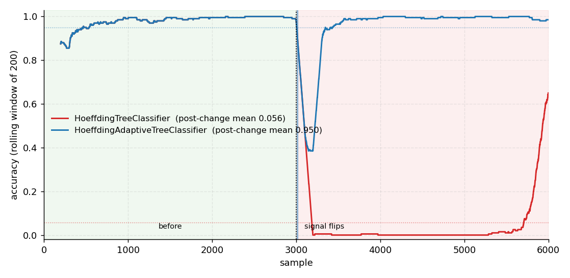
Over the 3000 samples after the change, the plain tree is right 5.6 % of the time (it keeps the
old answers); the adaptive tree detected the change (3 drift signals), swapped in its background
subtree once, and is right 95 % of the time. The swap test compares the errors of the two
subtrees counted on the same samples since the background one started, and swaps when the
difference exceeds $\sqrt{\ln(2/\delta)/n}$ after at least kappa_alt samples.
4. Predicting a number: the torque of a two-link arm
A regression tree that splits on the gradient of the loss (stochastic gradient tree): it predicts the gravity torque of the first joint of a two-link arm from the two joint angles.
import numpy as np
from dense_armor.utility.metrics import MeanAbsoluteError
from dense_armor.utility.tree import SGTRegressor

rng = np.random.default_rng(3)
sgt = SGTRegressor()
mae_sgt, mae_mean, mean, n = MeanAbsoluteError(), MeanAbsoluteError(), 0.0, 0
for _ in range(20000):
    q1, q2 = rng.uniform(-np.pi, np.pi, 2)
    tau = 9.81 * (2.0 * np.cos(q1) + np.cos(q1 + q2))
    x = {"q1": q1, "q2": q2}
    mae_sgt.update(tau, sgt.predict_one(x))
    mae_mean.update(tau, mean)
    sgt.learn_one(x, tau)
    n += 1
    mean += (tau - mean) / n
print(round(mae_sgt.get(), 3), round(mae_mean.get(), 3), sgt.n_nodes_)
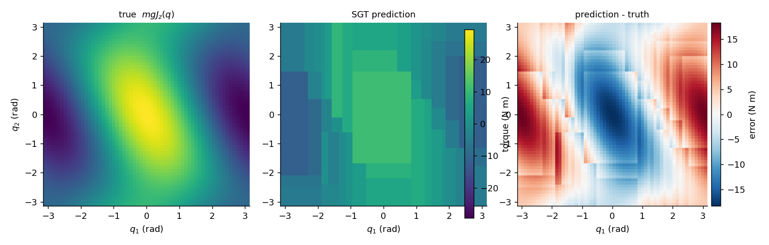
Tested before learning each sample, the tree's mean absolute error is 7.7 N·m against 13.2 N·m for the running mean, with 91 nodes. A split is made only when a t-test says the loss reduction is real (Gouk et al. 2019, eq. 16):
$$t = \frac{\bar L}{s / \sqrt{n}}$$
$\bar L$ is the mean change of the loss over the $n$ samples of the leaf, $s$ its standard
deviation; the split happens when the one-sided p-value is below delta (0.01). The variance of
each sample's change uses the gradient $G$, the Hessian $H$ and the value $v$ of the new leaf
(eq. 18):
$$\operatorname{Var}(L_i) = v^2 \operatorname{Var}(G) + \tfrac14 v^4 \operatorname{Var}(H) + v^3 \operatorname{Cov}(G, H)$$
5. A prediction with its uncertainty: Mondrian forests
A forest of 10 random trees that also says how sure it is; trained on joint positions between 0 and 1 only, it is asked inside and outside that range.
import numpy as np
from dense_armor.utility.tree import MondrianForestRegressor

rng = np.random.default_rng(4)
mf = MondrianForestRegressor(n_trees=10, seed=0)
for _ in range(1000):
    q = rng.uniform(0.0, 1.0)
    mf.learn_one({"q": q}, np.sin(6.0 * q) + rng.normal(0.0, 0.05))
for q in (0.5, 1.5, 3.0):
    e = mf.predict_one({"q": q}, return_estimate=True)
    print(q, round(e.mean, 3), round(e.std, 3))
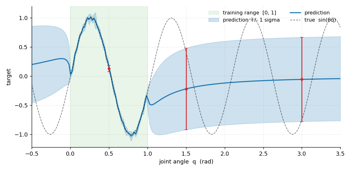
At q = 0.5 (inside the data) the prediction 0.131 is close to the true sin(3) = 0.141, with
standard deviation 0.054, about the noise of the data. Outside the data the standard deviation
jumps to 0.70: the forest says "I do not know", which a controller can use to slow down or ask
for help. Where it comes from: walking down a tree, a point outside a node's box "branches off"
before that node with probability (Lakshminarayanan et al. 2016, Algorithm 5)
$$p_j(x) = 1 - e^{-\Delta_j \eta_j(x)}, \qquad \Delta_j = \tau_j - \tau_{\mathrm{parent}(j)}$$
$\eta_j(x)$ is how far $x$ lies outside the box, $\tau$ the split times of the Mondrian process; the prediction is the mixture of the node statistics weighted by these probabilities (eq. 3), so the farther the point, the wider the mixture.
6. Which tree for which job
The same streams for every model, 4000 samples each, tested before learning each sample.
Classifiers see two features a, b; the target y is 0 or 1; a ~ N(3y, 0.5) and
b ~ N(0, 0.5); at sample 2000 a switches to N(3(1-y), 0.5). Regressors see two joint
angles q1, q2 ~ U(-pi, pi) and target tau = 9.81 (2 cos q1 + cos(q1+q2)) scaled by 1.0
before sample 2000 and 1.5 after. The script docs/assets/tree/make_table.py regenerates the
table below with these streams; ms per sample is measured on the machine that runs the
script.
| model | task | stationary | with a change | ms per sample |
|---|---|---|---|---|
HoeffdingTreeClassifier |
accuracy | 0.992 | 0.524 | 0.030 |
HoeffdingAnytimeTreeClassifier |
accuracy | 0.992 | 0.659 | 0.031 |
HoeffdingAdaptiveTreeClassifier (ADWIN) |
accuracy | 0.992 | 0.962 | 0.496 |
SGTClassifier |
accuracy | 0.842 | 0.773 | 0.061 |
MondrianForestClassifier |
accuracy | 0.998 | 0.605 | 1.272 |
SGTRegressor |
mean abs. error | 10.218 | 12.392 | 0.035 |
MondrianForestRegressor |
mean abs. error | 1.161 | 3.343 | 1.314 |
On a stable stream the three Hoeffding trees and the Mondrian forest classify almost perfectly; after a change, the adaptive tree recovers best among the trees, at about 16 times the cost per sample of the plain tree; the Mondrian forest is the most accurate regressor here and the only model with an uncertainty, at about 1 ms per sample; the stochastic gradient tree is the cheapest regressor. Accuracy "with a change" counts the whole stream, before and after the change.
API reference
hoeffding 
Hoeffding tree classifier.
A non-linear classifier that grows one sample at a time. Each leaf keeps enough statistics to estimate the information gain of a possible split; when the difference in gain between the best and the second-best candidate is larger than the Hoeffding bound, the leaf is split.
The Hoeffding bound of equation 1 of Manapragada et al. 2018 is
.. math::
\epsilon = \sqrt{\frac{R^2 \ln(1/\delta)}{2 n}}
where R is the range of the split-evaluation function (here
log2(K) for K classes), delta is one minus the required
confidence, and n is the number of samples seen at the leaf.
Numeric attributes are handled with a running Gaussian estimator per class and per feature inside each leaf. A candidate threshold is the midpoint between two consecutive class means; the fraction of each class on each side is estimated with the normal CDF.
Examples:
>>> import numpy as np
>>> from dense_armor.utility.tree.hoeffding import HoeffdingTreeClassifier
>>> rng = np.random.default_rng(0)
>>> h = HoeffdingTreeClassifier(grace_period=30)
>>> for _ in range(400):
...     x = float(rng.normal(0.0 if rng.random() < 0.5 else 5.0, 0.4))
...     y = 0 if x < 2.5 else 1
...     _ = h.learn_one({"x": x}, y=y)
>>> h.predict_one({"x": 0.1}) != h.predict_one({"x": 5.0})
True
References
Manapragada, C., Webb, G. I., Salehi, M. (2018). Extremely fast decision tree. In KDD. Domingos, P., Hulten, G. (2000). Mining high-speed data streams. In KDD.
HoeffdingTreeClassifier 
HoeffdingTreeClassifier(
    grace_period: int = 200,
    delta: float = 1e-07,
    tau: float = 0.05,
    max_depth: int | None = None,
    max_nodes: int | None = 10000,
    leaf: str = "nb",
)
Bases: Classifier
Hoeffding tree for incremental classification.
Memory grows with the number of nodes; max_nodes (default
10000) bounds the total, so memory_class is "O(window)".
budget_s = 1e-3 s: p99 of learn_one measured at 2.3e-5 s on a
2000-sample, two-feature stream on a desktop CPU (default
parameters); the budget leaves room for slower machines.
Parameters:
| Name | Type | Description | Default |
|---|---|---|---|
grace_period
|
int
|
minimum number of samples at a leaf before a split is attempted. |
200
|
delta
|
float
|
one minus the confidence of the Hoeffding bound. |
1e-07
|
tau
|
float
|
tie threshold. |
0.05
|
max_depth
|
int | None
|
maximum depth, or |
None
|
max_nodes
|
int | None
|
maximum number of nodes. Default |
10000
|
leaf
|
str
|
|
'nb'
|
Raises:
| Type | Description |
|---|---|
ValueError
|
on a bad |
Source code in dense_armor/utility/tree/hoeffding.py
learn_one 
Update the tree with one sample.
Source code in dense_armor/utility/tree/hoeffding.py
predict_proba_one 
Return the class-probability dict at the reached leaf.
Source code in dense_armor/utility/tree/hoeffding.py
predict_one 
Return the most likely class.
explain_one 
Return the path from root to leaf as a list of dicts.
Returns an empty list when the root itself is a leaf, that is when the tree never split from the root. This happens on small datasets where the Hoeffding bound (or the t-test for SGT) is never satisfied, so no split is statistically significant. The prediction is then a constant prior over the classes and there is no path to explain.
Source code in dense_armor/utility/tree/hoeffding.py
efdt 
Hoeffding Anytime Tree classifier.
The Hoeffding tree (Domingos and Hulten 2000) decides to split a leaf only when the best candidate attribute beats the second best by more than the Hoeffding bound, and it never revisits that decision. The Hoeffding Anytime Tree (HATT) of Manapragada et al. 2018 changes both points:
- a leaf splits as soon as the best candidate beats no split by more than the bound (Manapragada et al. 2018, Function 3.2);
- an internal node re-evaluates its own split every
grace_periodsamples that reach that node, and replaces the split when the best attribute beats the current one by more than the bound (Function 3.3). When no split is significantly better, the node becomes a leaf again.
Every node on the path of a sample updates its own sufficient
statistics in learn_one (Algorithm 3.1, the foreach node in
path loop).
Examples:
>>> import numpy as np
>>> from dense_armor.utility.tree.efdt import HoeffdingAnytimeTreeClassifier
>>> rng = np.random.default_rng(0)
>>> h = HoeffdingAnytimeTreeClassifier(grace_period=30)
>>> for _ in range(400):
...     x = float(rng.normal(0.0 if rng.random() < 0.5 else 5.0, 0.4))
...     y = 0 if x < 2.5 else 1
...     _ = h.learn_one({"x": x}, y=y)
>>> h.predict_one({"x": 0.1}) != h.predict_one({"x": 5.0})
True
References
Manapragada, C., Webb, G. I., Salehi, M. (2018). Extremely fast decision tree. In KDD, Algorithm 3.1, Functions 3.2 and 3.3. Domingos, P., Hulten, G. (2000). Mining high-speed data streams. In KDD.
HoeffdingAnytimeTreeClassifier 
HoeffdingAnytimeTreeClassifier(
    grace_period: int = 200,
    delta: float = 1e-07,
    tau: float = 0.05,
    max_depth: int | None = None,
    max_nodes: int | None = 10000,
    leaf: str = "nb",
)
Bases: HoeffdingTreeClassifier
Hoeffding Anytime Tree classifier.
Same interface and same leaf classifiers as
:class:HoeffdingTreeClassifier. Memory grows with the number of
nodes; max_nodes (default 10000) bounds the total.
budget_s = 1e-3 s: p99 of learn_one measured at 2.8e-5 s on a
2000-sample, two-feature stream on a desktop CPU (default
parameters); the budget leaves room for slower machines.
Parameters:
| Name | Type | Description | Default |
|---|---|---|---|
grace_period
|
int
|
minimum samples at a node before a split attempt and the interval between re-evaluations of an internal node. |
200
|
delta
|
float
|
one minus the confidence of the Hoeffding bound. |
1e-07
|
tau
|
float
|
tie threshold. |
0.05
|
max_depth
|
int | None
|
maximum depth, or |
None
|
max_nodes
|
int | None
|
maximum number of nodes. Default |
10000
|
leaf
|
str
|
|
'nb'
|
Raises:
| Type | Description |
|---|---|
ValueError
|
on a bad |
Source code in dense_armor/utility/tree/efdt.py
adaptive 
Hoeffding Adaptive Tree classifier.
The Hoeffding tree never revisits a split. The Hoeffding Adaptive Tree (HAT) of Bifet and Gavalda (2009) adds a drift detector at each node: when the detector warns, an alternate subtree grows in the background on the recent samples; when the alternate is significantly more accurate than the main one, it replaces the corresponding branch.
The detector and the error counters live on the node, not in a dict
keyed by id(node), so clone, pickle and state round-trips work.
Examples:
>>> import numpy as np
>>> from dense_armor.utility.drift.adwin import ADWIN
>>> from dense_armor.utility.tree.adaptive import HoeffdingAdaptiveTreeClassifier
>>> rng = np.random.default_rng(0)
>>> h = HoeffdingAdaptiveTreeClassifier(
...     grace_period=30, drift_detector=ADWIN()
... )
>>> for _ in range(400):
...     x = float(rng.normal(0.0 if rng.random() < 0.5 else 5.0, 0.4))
...     y = 0 if x < 2.5 else 1
...     _ = h.learn_one({"x": x}, y=y)
>>> h.predict_one({"x": 0.1}) != h.predict_one({"x": 5.0})
True
References
Bifet, A., Gavalda, R. (2009). Adaptive learning from evolving data streams. In IDA. Esteban, A., Cano, A., Zafra, A., Ventura, S. (2024). Hoeffding adaptive trees for multi-label classification on data streams. Domingos, P., Hulten, G. (2000). Mining high-speed data streams. In KDD.
HoeffdingAdaptiveTreeClassifier 
HoeffdingAdaptiveTreeClassifier(
    grace_period: int = 200,
    delta: float = 1e-07,
    tau: float = 0.05,
    max_depth: int | None = None,
    max_nodes: int | None = 10000,
    leaf: str = "nb",
    drift_detector: DriftDetector | None = None,
    delta_alt: float = 0.01,
    kappa_alt: int = 100,
    error_alpha: float = 0.005,
)
Bases: HoeffdingTreeClassifier
Hoeffding Adaptive Tree classifier.
Memory grows with the number of nodes of the main tree and of any
alternate subtrees; max_nodes (default 10000) bounds the
total.
budget_s = 5e-3 s: p99 of learn_one measured at 3.7e-4 s on a
2000-sample, two-feature stream on a desktop CPU (default
parameters); the budget leaves room for slower machines.
Parameters:
| Name | Type | Description | Default |
|---|---|---|---|
grace_period
|
int
|
minimum samples at a node before a split attempt. |
200
|
delta
|
float
|
one minus the confidence of the Hoeffding bound for splits. |
1e-07
|
tau
|
float
|
tie threshold. |
0.05
|
max_depth
|
int | None
|
maximum depth, or |
None
|
max_nodes
|
int | None
|
maximum number of nodes. Default |
10000
|
leaf
|
str
|
|
'nb'
|
drift_detector
|
DriftDetector | None
|
a fresh |
None
|
delta_alt
|
float
|
one minus the confidence of the alternate bound. |
0.01
|
kappa_alt
|
int
|
minimum samples for an alternate to be considered. |
100
|
error_alpha
|
float
|
smoothing of the per-node error estimate. |
0.005
|
Raises:
| Type | Description |
|---|---|
ValueError
|
on a bad |
Source code in dense_armor/utility/tree/adaptive.py
sgt 
Stochastic gradient trees for regression and classification.
An incremental decision tree built from stochastic gradient information. Each node keeps the sums of the first and second derivatives of the loss with respect to the current prediction; a candidate split is scored with the reduction of the quadratic Taylor expansion of the loss (equation 7 of Gouk et al. 2019), the optimal value of a new leaf is the Newton step of equation 13, and a t-test in place of the Hoeffding bound decides whether to split (equation 16).
For regression the loss is the squared error, whose first and second
derivatives with respect to the prediction are g = y_hat - y and
h = 1 (equations 24-25). For binary classification the loss is the
logistic log loss with a single logistic output; the first derivative
is g = p - y and the second is h = p (1 - p) where
p = sigmoid(f(x)).
Examples:
>>> from dense_armor.utility.tree.sgt import SGTRegressor
>>> s = SGTRegressor(min_samples_split=20, n_bins=16, bin_samples=50)
>>> for i in range(2000):
...     x = (i % 50) / 49.0
...     _ = s.learn_one({"x": x}, y=x)
>>> s.n_seen_ > 0 and s.n_nodes_ > 1
True
References
Gouk, H., Pfahringer, B., Frank, E. (2019). Stochastic gradient trees. In ACML, sections 3.1-3.3.
SGTRegressor 
SGTRegressor(
    delta: float = 0.01,
    min_samples_split: int = 50,
    grace_period: int = 200,
    n_bins: int = 64,
    bin_samples: int = 1000,
    lambda_: float = 0.1,
    gamma: float = 1.0,
    max_depth: int | None = None,
    max_nodes: int | None = 10000,
)
Bases: Regressor, _SGTBase
Stochastic gradient tree for regression.
Minimises the squared loss by taking one Newton step per update.
The split is accepted when the one-sided p-value of the t-test of
section 3.3 is below delta.
Memory grows with the number of nodes; max_nodes (default
10000) bounds the total, so memory_class is "O(window)".
Parameters:
| Name | Type | Description | Default |
|---|---|---|---|
delta
|
float
|
one minus the confidence of the t-test. |
0.01
|
min_samples_split
|
int
|
minimum samples at a leaf before a split. |
50
|
grace_period
|
int
|
interval in samples between two split attempts. |
200
|
n_bins
|
int
|
number of equal-width bins per numeric feature. |
64
|
bin_samples
|
int
|
initial samples used to estimate feature ranges. |
1000
|
lambda_
|
float
|
L2 penalty on the leaf values. |
0.1
|
gamma
|
float
|
cost per new node. |
1.0
|
max_depth
|
int | None
|
maximum depth, or |
None
|
max_nodes
|
int | None
|
maximum number of nodes. Default |
10000
|
Raises:
| Type | Description |
|---|---|
ValueError
|
on a non-positive parameter. |
budget_s = 1e-3 s: p99 of learn_one measured at 1.2e-5 s on a
2000-sample, two-feature stream on a desktop CPU (default
parameters); the budget leaves room for slower machines.
Source code in dense_armor/utility/tree/sgt.py
learn_one 
Update the tree with one sample.
Source code in dense_armor/utility/tree/sgt.py
predict_one 
Return the predicted value at the reached leaf.
Source code in dense_armor/utility/tree/sgt.py
explain_one 
Return the path from root to leaf as a list of dicts.
Returns an empty list when the root itself is a leaf, that is when the tree never split from the root. This happens on small datasets where the t-test on the loss reduction (Gouk et al. 2019, eq. 16) never accepts a split. The prediction is then a constant Newton step at the root and there is no path to explain.
Source code in dense_armor/utility/tree/sgt.py
SGTClassifier 
SGTClassifier(
    delta: float = 0.01,
    min_samples_split: int = 50,
    grace_period: int = 200,
    n_bins: int = 64,
    bin_samples: int = 1000,
    lambda_: float = 0.1,
    gamma: float = 1.0,
    max_depth: int | None = None,
    max_nodes: int | None = 10000,
)
Bases: Classifier, _SGTBase
Stochastic gradient tree for binary classification.
A single logistic output, p = sigmoid(f(x)), is trained with
the logistic log loss. The split is accepted when the one-sided
p-value of the t-test of section 3.3 is below delta.
Memory grows with the number of nodes; max_nodes (default
10000) bounds the total, so memory_class is "O(window)".
Parameters:
| Name | Type | Description | Default |
|---|---|---|---|
delta
|
float
|
one minus the confidence of the t-test. |
0.01
|
min_samples_split
|
int
|
minimum samples at a leaf before a split. |
50
|
grace_period
|
int
|
interval in samples between two split attempts. |
200
|
n_bins
|
int
|
number of equal-width bins per numeric feature. |
64
|
bin_samples
|
int
|
initial samples used to estimate feature ranges. |
1000
|
lambda_
|
float
|
L2 penalty on the leaf values. |
0.1
|
gamma
|
float
|
cost per new node. |
1.0
|
max_depth
|
int | None
|
maximum depth, or |
None
|
max_nodes
|
int | None
|
maximum number of nodes. Default |
10000
|
Raises:
| Type | Description |
|---|---|
ValueError
|
on a non-positive parameter. |
budget_s = 1e-3 s: p99 of learn_one measured at 2.4e-5 s on a
2000-sample, two-feature stream on a desktop CPU (default
parameters); the budget leaves room for slower machines.
Source code in dense_armor/utility/tree/sgt.py
learn_one 
Update the tree with one sample.
Source code in dense_armor/utility/tree/sgt.py
predict_proba_one 
Return the class-probability dict.
Source code in dense_armor/utility/tree/sgt.py
predict_one 
Return the most likely class.
mondrian 
Online Mondrian forests for regression and classification.
A Mondrian process (Roy and Teh 2009) is a random hierarchical partition of the input space whose splits occur at exponentially distributed times, with rate equal to the sum of the extents of the block being split. A Mondrian tree is the restriction of a Mondrian process to a finite set of points: the tree is finite, the split dimension is chosen with probability proportional to the extent of the block along that dimension, and the split location is uniform in that extent. This is the tree distribution of Lakshminarayanan et al. 2014 (classification) and 2016 (regression).
The online extension follows Algorithms 3 and 4 of the 2014 paper: when a new point falls outside a node's data extent, an additional split above that node is sampled with rate equal to the extent extension; the dimension is chosen with probability proportional to its extension and the cut is uniform in it.
A forest is a collection of independent Mondrian trees. The prediction of the forest averages the tree predictions. For regression, each tree returns a Gaussian mixture over the labels (2016, eq. 3): along the path from the root to the leaf that contains the query point, the probability of branching off just before each node contributes the weight of that node's posterior. The predictive variance is the mixture variance, so it grows as the query moves away from the training data.
Examples:
>>> from dense_armor.utility.tree.mondrian import MondrianForestRegressor
>>> f = MondrianForestRegressor(n_trees=5, seed=0)
>>> for i in range(500):
...     x = (i % 50) / 49.0
...     _ = f.learn_one({"x": x}, y=x)
>>> e = f.predict_one({"x": 0.5}, return_estimate=True)
>>> e.var >= 0.0
True
References
Lakshminarayanan, B., Roy, D. M., Teh, Y. W. (2014). Mondrian forests: efficient online random forests. In NIPS, section 2, section 3.1, Algorithms 2, 3 and 4. Lakshminarayanan, B., Roy, D. M., Teh, Y. W. (2016). Mondrian forests for large-scale regression when uncertainty matters. In AISTATS, section 3, eq. 3. Roy, D. M., Teh, Y. W. (2009). The Mondrian process. In NIPS.
MondrianForestRegressor 
MondrianForestRegressor(
    n_trees: int = 10,
    lifetime: float = math.inf,
    max_nodes: int | None = 10000,
    seed: int = 0,
)
Bases: Regressor, _MondrianBase
Online Mondrian forest for regression.
Prediction is the mean of the per-tree Gaussian posteriors; the
predictive variance is the mixture variance of eq. 3 of
Lakshminarayanan et al. 2016, so it grows as the query point moves
away from the training data. Memory grows with the number of nodes
in the forest; max_nodes (default 10000) bounds each tree.
budget_s = 2e-2 s: p99 of learn_one measured at 1.3e-3 s on a
2000-sample, two-feature stream on a desktop CPU (default
parameters); the budget leaves room for slower machines.
Parameters:
| Name | Type | Description | Default |
|---|---|---|---|
n_trees
|
int
|
number of trees in the forest. |
10
|
lifetime
|
float
|
lifetime parameter of the Mondrian process. |
inf
|
max_nodes
|
int | None
|
maximum number of nodes per tree. Default |
10000
|
seed
|
int
|
base random seed; tree |
0
|
Raises:
| Type | Description |
|---|---|
ValueError
|
on a non-positive parameter . |
Source code in dense_armor/utility/tree/mondrian.py
learn_one 
Update every tree with one sample.
Source code in dense_armor/utility/tree/mondrian.py
predict_one 
predict_one(
    x: Any,
    t: float | None = None,
    return_std: bool = False,
    return_estimate: bool = False,
) -> Any
Return the predictive mean, and the variance on request.
Source code in dense_armor/utility/tree/mondrian.py
MondrianForestClassifier 
MondrianForestClassifier(
    n_trees: int = 10,
    lifetime: float = math.inf,
    max_nodes: int | None = 10000,
    seed: int = 0,
)
Bases: Classifier, _MondrianBase
Online Mondrian forest for classification.
Each tree predicts a smoothed distribution at the leaf that
contains the query point: counts along the path are weighted by
the probability of branching off just before each node. The forest
averages the per-tree distributions. Memory grows with the number
of nodes; max_nodes (default 10000) bounds each tree.
budget_s = 2e-2 s: p99 of learn_one measured at 1.6e-3 s on a
2000-sample, two-feature stream on a desktop CPU (default
parameters); the budget leaves room for slower machines.
Parameters:
| Name | Type | Description | Default |
|---|---|---|---|
n_trees
|
int
|
number of trees in the forest. |
10
|
lifetime
|
float
|
lifetime parameter of the Mondrian process. |
inf
|
max_nodes
|
int | None
|
maximum number of nodes per tree. Default |
10000
|
seed
|
int
|
base random seed; tree |
0
|
Raises:
| Type | Description |
|---|---|
ValueError
|
on a non-positive parameter . |
Source code in dense_armor/utility/tree/mondrian.py
learn_one 
Update every tree with one sample.
Source code in dense_armor/utility/tree/mondrian.py
predict_proba_one 
Return the class probabilities from the forest.
Source code in dense_armor/utility/tree/mondrian.py
predict_one 
Return the most likely class.
Details
- Hoeffding tree: each leaf keeps a Gaussian per class and feature; candidate thresholds are
midpoints between consecutive class means; leaves predict with naive Bayes (
leaf="nb") or the majority class;tau(0.05) is the tie threshold. Domingos and Hulten (2000) introduced the tree; the bound and the Anytime variant are from Manapragada et al. (2018), Algorithm 3.1, Functions 3.2 and 3.3. - Adaptive tree: a detector on each internal node (default
ADWIN, cloned per node); swap and discard are decided only afterkappa_alt(100) samples of the background subtree, on errors counted on the same samples. As in Esteban et al. (2024), the detectors sit on the internal nodes. - Stochastic gradient trees: features are cut into 64 equal-width bins, their range estimated on
the first 1000 samples (section 3.2); per-bin moments of gradient and Hessian are merged with
the pairwise update before eq. 18; the t distribution is computed with the regularized
incomplete beta function, no external library at runtime;
SGTClassifieris binary. - Mondrian forests: split times follow Algorithm 2 (leaves have time equal to the lifetime) and
new points extend the tree with Algorithm 4 of the 2014 paper, so online and batch trees have
the same distribution (eq. 1 there); every node keeps the statistics of its block. With the
default lifetime (infinite) a tree keeps growing until
max_nodes. Departure from the paper: classification uses normalised class histograms in the mixture instead of the hierarchical smoothing of the paper, and blocks are not paused when their labels are all identical. - Every class caps its size with
max_nodes(default 10000), so memory is bounded;budget_sis about ten times the 99th percentile oflearn_onemeasured on a desktop CPU. - Figures on this page are generated by
docs/assets/tree/make_figure.py. - Sources: Manapragada, C., Webb, G. I., Salehi, M. (2018), "Extremely fast decision tree", arXiv:1802.08780. Esteban, A., Cano, A., Zafra, A., Ventura, S. (2024), "Hoeffding adaptive trees for multi-label classification on data streams", arXiv:2410.20242. Gouk, H., Pfahringer, B., Frank, E. (2019), "Stochastic gradient trees", arXiv:1901.07777. Lakshminarayanan, B., Roy, D. M., Teh, Y. W. (2014), "Mondrian forests: efficient online random forests", arXiv:1406.2673; (2016) "Mondrian forests for large-scale regression when uncertainty matters", arXiv:1506.03805.