LODA

LODA tells you when a new reading from your robot looks strange. It looks at the numbers from many different points of view: each one squeezes the readings into a single number and keeps a tally of the values it saw recently. A new reading that lands on a value almost never seen looks strange from that point of view. LODA averages all the points of view and gives back a score: the higher it is, the stranger the reading.

LODA scores each sample by how rare its position is in a few random one-dimensional projections of the joint residual. In a control loop it answers one question per reading: does this residual land in a part of the space the healthy run almost never visits?

1. What it is

A robot produces, per joint, a torque residual — the difference between the measured torque and the torque the URDF model predicts. On a healthy arm this residual stays within a narrow band. When something changes (a payload, a worn bearing, a slack cable), the residual moves to a region of the d-dimensional joint space that the healthy arm rarely or never visits.

LODA looks at each joint-space point through many random 1-D projections: it draws a direction, projects every sample onto it, and histograms the projection values over a sliding window. A sample that falls in a bin the window rarely visits gets a high anomaly score. Averaging the score across the projections gives the final number.

The idea is that some fault directions are visible in one projection and invisible in another. A single histogram over the raw d-dimensional space would need an exponential number of bins; d-dimensional histograms over many 1-D projections need a linear number.

2. How it works

For each of n_projections random directions w_j, the detector normalises the sample feature by feature,

x_norm = (x - lo) / (hi - lo)

with lo and hi the working ranges of the features (learned from the first range_init samples, or given as feature_ranges), and then projects it onto the direction:

proj_j = <w_j, x_norm>

Because w_j is L2-normalised with k Gaussian non-zero entries and x_norm lives in [0, 1]^d, the projection is bounded by the theoretical interval [pmin_j, pmax_j], where pmin_j is the sum of the negative entries of w_j and pmax_j the sum of the positive ones. That interval spreads the projections over all the bins: the bin index is

bin_j = floor(n_bins * (proj_j - pmin_j) / (pmax_j - pmin_j))

clipped to [0, n_bins - 1]. The counts of the bins are updated every sample inside a sliding window of the last window samples.

The score of a sample is the mean over the projections of

-log2( (c_bin + 1) / (N + 1) )

where c_bin is the count in the bin the projection falls into, and N is the total number of samples currently in the window. A rare bin (c_bin = 0) gives a high score; a common one gives a low score.

The projections are sparse: each w_j has only max(1, d // 2) non-zero entries, so a projection mixes only half of the features. Different projections mix different subsets, which gives the ensemble its diversity.

The + 1 on both sides of the ratio keeps the score finite on empty bins and empty windows. With window = 200 and an empty bin, the score saturates at log2(201) ~= 7.65.

The implementation follows Lou et al. (2024), fSEAD, section on Loda: random projection of the input, one histogram per projection, score -mean(log2(c / W)). The original LODA paper is Pevny (2016), whose Eq. 3 is f(x) = -mean_i(log h_i(x)) with log natural and h_i(x) the histogram probability. The implementation uses log2 and a +1 smoothing on numerator and denominator. The base change is a constant factor that does not affect the ordering of the scores; the smoothing keeps the first samples from scoring infinite.

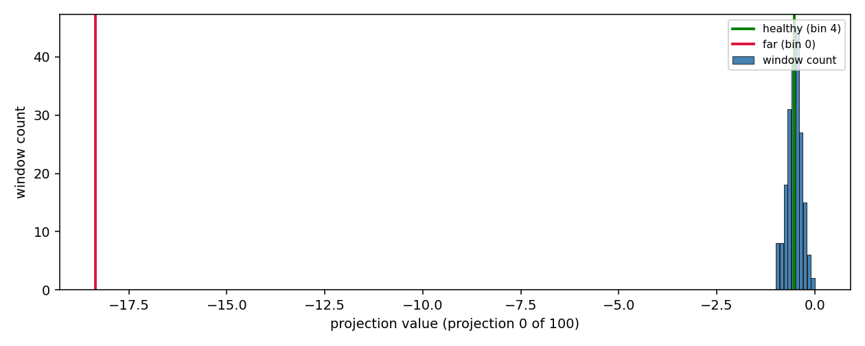
One of the hundred projections. The blue bars are the counts of the sliding window; the green line is where a healthy sample falls; the red line is where an out-of-distribution sample falls. The healthy one lands in a bin with hundreds of samples, the anomaly in a bin the window never visits.

3. Smallest example

import numpy as np
from dense_armor.utility.anomaly.loda import LODA

rng = np.random.default_rng(0)
det = LODA(n_projections=50, n_bins=10, window=200, range_init=50, seed=0)

for _ in range(300):
    det.learn_one({
        "a": float(rng.normal(0.5, 0.05)),
        "b": float(rng.normal(0.5, 0.05)),
    })

print(f"healthy      {det.score_one({'a': 0.5, 'b': 0.5}):.3f}")
print(f"far outlier  {det.score_one({'a': 5.0, 'b': 5.0}):.3f}")

healthy      2.380
far outlier  4.648

The healthy point sits where the healthy samples sit, and falls in bins the window visits often, so its score is low. The far point is outside the working range and is clipped to the outermost bin of every projection; those bins are the ones the window almost never visits, so the score rises to 4.648. That value is below log2(201) = 7.651, the score of an empty bin in every projection, because some projections still land the far point in a bin the window visits.

4. On a real arm

The residual of joints 1-4 on a SyntheticArm payload fault. The fault (5 kg added at t = 2 s) shifts the residual on joints 1-5 by tens of N·m; the healthy run stays within ±0.15 N·m.

from pathlib import Path
from dense_armor.utility.anomaly.loda import LODA
from dense_armor.utility.datasets import SyntheticArm

ds = SyntheticArm(
    Path("test/fixtures/urdf/panda.urdf"),
    period_s=2.0, rate_hz=50.0, n_cycles=4,
    fault_at_s=2.0, fault="payload", payload_mass=5.0,
    noise_std=(1e-3, 5e-3, 5e-2), seed=0,
)

det = LODA(
    n_projections=100, n_bins=10, window=200, range_init=50,
    feature_keys=["r0", "r1", "r2", "r3"], threshold=4.0, seed=0,
)

for sig, _ in ds.stream():
    q, qd, qdd = ds.trajectory(sig.t)
    tau_nom = ds.nominal_torque(q, qd, qdd)
    x = {f"r{j}": float(sig[f"tau_{j}"] - tau_nom[j]) for j in range(4)}
    _ = det.score_one(x)
    _ = det.learn_one(x)

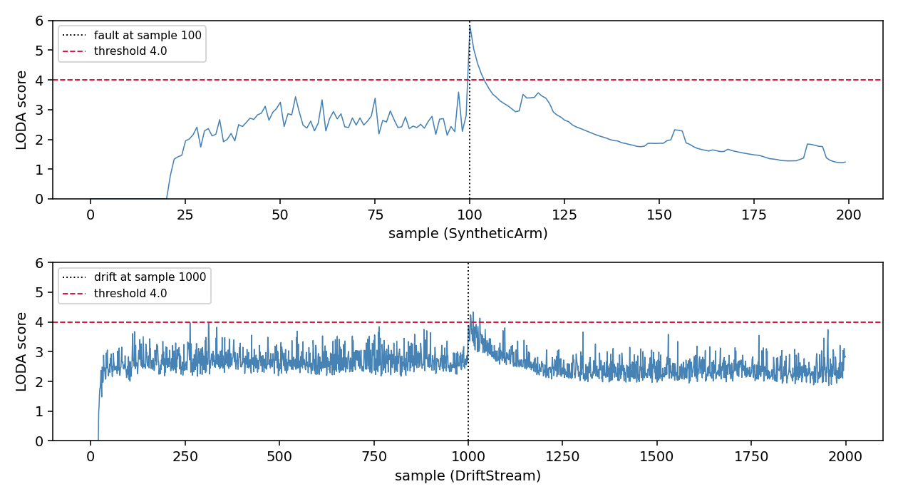
Top: SyntheticArm, the fault shifts the residual to bins the healthy run never visited. Bottom: DriftStream with one sudden drift at the half of the stream. Both score the change above the threshold (4.0) on nearly every post-change sample, with no false alarms on the healthy part.

5. Numbers

SyntheticArm (200 samples, 100 healthy, 100 fault) and DriftStream (2000 samples, one sudden drift at half), every detector built with its defaults.

Stream	Protocol	ROC-AUC	False alarms on the healthy part	Threshold at the last healthy sample
SyntheticArm	learn-on-healthy	1.000	0.000	4.0000
SyntheticArm	learn-on-all	0.456	0.000	4.0000
DriftStream	learn-on-healthy	0.989	0.000	4.0000
DriftStream	learn-on-all	0.332	0.000	4.0000

The two streams are the same used for every other detector on this page. LODA reaches the best ROC-AUC on the arm among the tree and projection detectors (1.000 learn-on-healthy) and stays above 0.98 on the drift stream, at 0.525 ms per sample on the arm with the benchmark defaults.

Details

References

Lou, B., Boland, D., Leong, P. H. W. (2024). fSEAD: a Composable FPGA-based Streaming Ensemble Anomaly Detection Library. arXiv:2406.05999. Section 2.1 (Streaming Anomaly Detection, Loda), Algorithm 1 line 14.

Pevny, T. (2016). LODA: Lightweight on-line detector of anomalies. Machine Learning 102(2), 275-304. Eq. 3.

Choices stated explicitly

• Projection. Sparse random Gaussian vector with k non-zero entries, chosen uniformly without replacement, L2-normalised. k = max(1, d // 2) by default. The paper writes -log2(v); the sign is inverted here so that a high score means anomalous, the convention of AnomalyDetector.
• Histogram. The projection is mapped to [0, 1] with its theoretical minimum and maximum before the bin is chosen: pmin_j the sum of the negative entries of w_j and pmax_j the sum of the positive ones. Lou et al. (Algorithm 1, line 14) write (prj_X - loda_min) / (loda_max - loda_min) without defining loda_min and loda_max; this implementation uses the theoretical interval above, because minimum and maximum observed on the window would make the bin depend on the order of the samples. When feature_ranges is None, the first range_init samples set the working range (min and max per feature, with a 10 % margin).
• Defaults. Lou et al. use 20 bins and a window of 128 (Table 4); the defaults here are n_bins=10 and window=256; the difference is a choice of this implementation.
• Score. mean(-log2((c + 1) / (W + 1))) over the projections. The + 1 on both sides smooths empty bins and empty windows, so the score stays finite.
• Threshold. A single float (default 4.0), because the score is bounded in [0, log2(window + 1)] and the natural flagging level depends on the window size. No adaptive quantile here: the score is already a log-likelihood.

Measured cost

At the benchmark defaults (n_projections=100, n_bins=10, window=256, range_init=20), on one CPU thread:

• 0.525 ms per sample for learn_one + score_one on the arm stream (learn-on-healthy, 100 healthy samples) and 0.609 ms on DriftStream;
• memory flat: 100 * 10 counters + window * n_projections bin indices, independent of the stream length.

The budget_s declared by the class is 0.002 s.

What the detector does not do

It counts bins, it does not model the joint distribution. A fault that moves the residual along a direction that no projection sees can hide. n_projections and n_bins trade accuracy for cost: with ten projections and four bins the score is noisy; with five hundred and thirty-two it is stable but costs proportionally. The defaults target a few hundred samples per window.

OnlineRobustMahalanobis is the alternative when the fault is a shift of the mean rather than a rare bin.