Robust statistics

The average can be pulled far off by one bad reading; the middle value (the median) cannot. These tools compute summary numbers that a few bad readings cannot spoil.

What this is

A robot has a temperature sensor on its shoulder. The sensor is usually accurate, but once every few minutes it glitches and reports a value fifty degrees higher than the real one. If you compute the mean of the last hundred readings, the glitch pulls the average up by half a degree, and it takes another hundred clean readings before the mean returns to where it was.

The mean is not robust: a single bad sample can move it as much as it wants. The median is: a single bad sample cannot move it at all, as long as fewer than half of the samples are bad.

This module computes the robust statistics of a stream — median, median absolute deviation, interquartile range, arbitrary quantile — over a bounded window. A window is a small number of the most recent samples. Memory stays fixed, cost per sample stays fixed, and the statistic is not affected by isolated outliers.

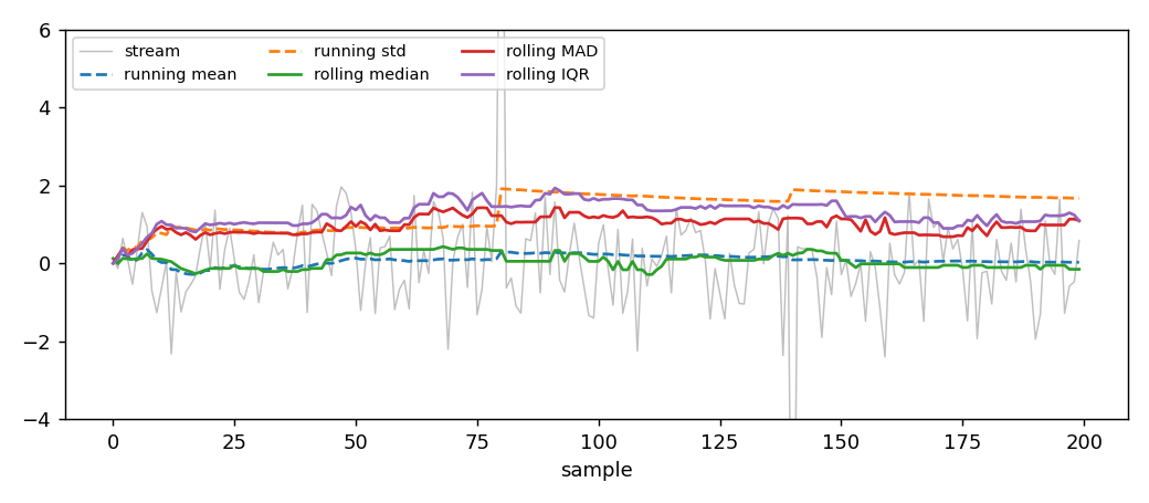
The figure shows a short stream of two hundred Gaussian samples with two large spikes injected at samples 80 and 140. The running mean jumps at each spike and takes many samples to recover. The rolling median, the rolling MAD and the rolling IQR do not move.

1. The first estimator

RollingMedian keeps the last window samples in a small queue and answers with their median.

from dense_armor.utility.stats.robust import RollingMedian

m = RollingMedian(window=5)
for v in [3.0, 1.0, 4.0, 1.0, 5.0, 9.0, 2.0]:
    m.learn_one({"x": v})
print(m.value)

The output is 4.0. After the seven samples, the window holds the five most recent values [1.0, 5.0, 9.0, 2.0, ...] — actually the last five of the input, which are [4.0, 1.0, 5.0, 9.0, 2.0]. Sorted, those are [1.0, 2.0, 4.0, 5.0, 9.0], and their median is 4.0.

The dict {"x": v} is one sample. The smallest key is read by default; RollingMedian(feature="temperature") names a specific one.

2. What a window is

The window is a FIFO queue of fixed length. When a new sample arrives and the queue is full, the oldest sample is dropped and the new one is added.

from dense_armor.utility.stats.robust import RollingMedian

m = RollingMedian(window=5)
for v in [3.0, 1.0, 4.0, 1.0, 5.0, 9.0, 2.0]:
    m.learn_one({"x": v})
print(m.value)
m = RollingMedian(window=3)
for v in [10.0, 20.0, 30.0, 1.0]:
    m.learn_one({"x": v})
print(m.value)

The output is 20.0. The window went from [10, 20, 30] to [20, 30, 1]; sorted, [1, 20, 30]; median 20.0.

The window can also be given in seconds, using the timestamps:

from dense_armor.utility.stats.robust import RollingMedian

m = RollingMedian(window=5)
for v in [3.0, 1.0, 4.0, 1.0, 5.0, 9.0, 2.0]:
    m.learn_one({"x": v})
print(m.value)
m = RollingMedian(window=3)
for v in [10.0, 20.0, 30.0, 1.0]:
    m.learn_one({"x": v})
print(m.value)
m = RollingMedian(window_s=0.05)
for i in range(100):
    m.learn_one({"x": float(i)}, t=i * 0.01)
print(m.window_size)

The output is 5. At 100 Hz (one sample every 0.01 seconds), half a second contains five samples. The base keeps the median inter-sample interval dt and converts a window in seconds to a number of samples automatically. Before two timestamps have been seen, dt is None and the window falls back to whatever window was set to.

3. Why the median is robust

Take a stream of numbers. The mean is the sum divided by the count. The median is the value that sits in the middle when the samples are sorted: half are smaller, half are larger. For an odd count, the median is one of the samples; for an even count, it is halfway between the two central ones.

The formulas, for a sample x₁ ≤ x₂ ≤ … ≤ xₙ sorted:

$$ \text{median} = \begin{cases} x_{(n+1)/2} & n \text{ odd}, \[4pt] \tfrac{1}{2}\left(x_{n/2} + x_{n/2+1}\right) & n \text{ even}. \end{cases} $$

The median is robust because a single large value only changes which rank it occupies: it moves to one end of the sorted list and the middle does not move.

The price of robustness is that the median ignores information. If you have [1, 2, 3, 4, 1000], the mean is 202 and the median is 3. The median says "the typical value is 3", which is true; the mean is dragged by the outlier.

4. Measuring the wobble: MAD

Once you have the median, you need a scale — a number that says how much the stream wobbles around the median. The natural robust choice is the median absolute deviation:

$$ \text{MAD} = \operatorname{median}!\left(\left|x_i - \operatorname{median}(x)\right|\right). $$

In words: compute the deviation of every sample from the median, take the absolute value of each, and take the median of those absolute deviations. The result is a scale in the same units as the data.

For Gaussian data, the MAD is about 0.6745 σ, not σ. To make the MAD comparable to the standard deviation of a Gaussian, multiply by the constant

$$ 1 / 0.6745 \approx 1.4826. $$

This is the value of MAD_SCALE in the module, and it is what RollingMAD.value returns by default. The constant was popularised by Hampel (1974). If you want the raw MAD without the scaling, pass scale=1.0:

from dense_armor.utility.stats.robust import RollingMAD

m = RollingMAD(window=5, scale=1.0)
for v in [1.0, 2.0, 3.0, 4.0, 5.0]:
    m.learn_one({"x": v})
print(m.value)

The output is 1.0, the raw MAD.

5. A hand case: MAD on five samples

Take [1, 2, 3, 4, 5]. The median is 3. The deviations from the median are |1−3|=2, |2−3|=1, |3−3|=0, |4−3|=1, |5−3|=2. Sorted: [0, 1, 1, 2, 2]. The median of those is 1. The default RollingMAD multiplies by 1.4826:

from dense_armor.utility.stats.robust import RollingMAD

m = RollingMAD(window=5)
for v in [1.0, 2.0, 3.0, 4.0, 5.0]:
    m.learn_one({"x": v})
print(round(m.value, 4))

The output is 1.4826. The raw MAD is 1; the scaled MAD is 1.4826. Both are useful: the raw one for the "middle spread of the middle 50%", the scaled one for comparing to a Gaussian standard deviation.

6. Measuring the spread: IQR

Another robust scale is the interquartile range, the difference between the 75th and the 25th percentile:

$$ \text{IQR} = Q_{0.75} - Q_{0.25}. $$

For Gaussian data, the IQR is about 1.349 σ, so dividing by that constant gives a scale comparable to σ. The module provides the raw IQR by default and the sigma-equivalent scale on request:

from dense_armor.utility.stats.robust import IQR_SCALE, RollingIQR

m = RollingIQR(window=5, scale=IQR_SCALE)
for v in [1.0, 2.0, 3.0, 4.0, 5.0]:
    m.learn_one({"x": v})
print(round(m.value, 4))

The output is 2.0. The raw IQR of [1..5] is Q3 − Q1 = 4 − 2 = 2. Multiplying by IQR_SCALE = 1 / 1.349 ≈ 0.7413 would give 1.4826, the same as the scaled MAD — which is exactly what you would expect for a Gaussian sample.

Which one to use

• MAD — easier to defend as a scale ("how much do the deviations from the median wobble?"). Its Gaussian scale factor is 1.4826.
• IQR — easier to explain as a spread ("how wide is the middle half of the data?"). Its Gaussian scale factor is 1 / 1.349 ≈ 0.7413.

Both are robust to outliers. The MAD is slightly more sensitive to the tails; the IQR slightly less.

7. Any quantile, not just the median

The 50th percentile is the median. The 90th percentile is what a service-level agreement usually refers to ("99% of requests under 200 ms"). RollingQuantile gives any q between 0 and 1, using the same linear interpolation as numpy.percentile.

from dense_armor.utility.stats.robust import RollingQuantile

m = RollingQuantile(q=0.9, window=5)
for v in [1.0, 2.0, 3.0, 4.0, 5.0]:
    m.learn_one({"x": v})
print(m.value)

The output is 4.6. The sorted window is [1, 2, 3, 4, 5]. The position for q = 0.9 over 5 samples is 0.9 × (5 − 1) = 3.6. The integer part is 3, the fractional part is 0.6. The value is x[3] + 0.6 · (x[4] − x[3]) = 4 + 0.6 = 4.6.

For q = 0.5, RollingQuantile returns exactly the same value as RollingMedian. The two are interchangeable at q = 0.5.

8. All joints at once

A robot has many joints. RollingMedianVector keeps one rolling median per channel and updates all of them from a single dict.

from dense_armor.utility.stats.robust import RollingMedianVector

v = RollingMedianVector(window=3)
for q in ([0.1, 0.2], [0.12, 0.18], [0.11, 0.21], [0.09, 0.19]):
    v.learn_one({"q0": q[0], "q1": q[1]})
summary = v.transform_one({})
print(round(summary["q0"]["value"], 4), round(summary["q1"]["value"], 4))

The output is 0.11 0.19. Each channel keeps its own window of three samples, so the median of joint 0 is the median of the last three q0 values, and similarly for joint 1.

9. A stream from a robot

A joint stream arrives as a sequence of standard joint-state readings: positions q, velocities qd, torques tau. Rolling medians are the right filter when the stream contains occasional spikes that must be ignored but not removed.

from dense_armor.utility.learn.online_dynamics import write_minimal_urdf
from dense_armor.dynamics.urdf_dynamics import RigidBodyModel
from dense_armor.utility.stats.robust import RollingMedianVector

model = RigidBodyModel(write_minimal_urdf())
import numpy as np
rng = np.random.default_rng(0)
stream = [tuple(rng.uniform(-1, 1, (3, model.n))) for _ in range(200)]
filtered = RollingMedianVector(window=5)
for i, (q, qd, tau) in enumerate(stream):
    readings = {f"q{j}": float(q[j]) for j in range(model.n)}
    filtered.learn_one(readings, t=i * 0.01)
summary = filtered.transform_one({})

After the loop, summary["q0"]["value"] is the median of the last five positions of joint 0. A spike in q0 at the end of the stream does not move the answer, as long as the spike is shorter than half the window.

The window is five samples by default; for a control loop at 1 kHz that is 5 milliseconds. Passing window_s=0.05 would use the timestamps to choose 50 samples instead.

10. Peak-to-peak, minimum and maximum

Every rolling robust statistic also carries the number of samples seen and the number of NaN samples skipped:

from dense_armor.utility.stats.robust import RollingMedian

m = RollingMedian(window=5)
for v in [3.0, 1.0, 4.0, 1.0, 5.0, 9.0, 2.0]:
    m.learn_one({"x": v})
print(m.value)
m = RollingMedian(window=3)
for v in [10.0, 20.0, 30.0, 1.0]:
    m.learn_one({"x": v})
print(m.value)
m = RollingMedian(window_s=0.05)
for i in range(100):
    m.learn_one({"x": float(i)}, t=i * 0.01)
print(m.window_size)
m = RollingMedian(window=5)
for v in [1.0, float("nan"), 3.0, float("nan"), 5.0]:
    m.learn_one({"x": v})
print(m.count, m.n_missing, m.value)

The output is 3 2 3.0. Three valid samples, two skipped, and the median of the valid ones. A sensor glitch does not corrupt the window; it bumps a counter.

Details

Reference formulas

• Tukey, J. W. (1977). Exploratory Data Analysis. Addison-Wesley — the interquartile range and the median-based view of robustness.
• Hampel, F. R. (1974). The influence curve and its role in robust estimation. Journal of the American Statistical Association 69(346), 383–393 — the median absolute deviation and the 1.4826 scale constant.
• Hyndman, R. J., Fan, Y. (1996). Sample quantiles in statistical packages. The American Statistician 50(4), 361–365 — the type 7 quantile interpolation used by numpy.percentile and by this module.

Where the classes live

• RollingMedian(window=20, window_s=None, feature=None) — median of the last window.
• RollingMAD(window=20, window_s=None, feature=None, scale=1.4826) — scaled median absolute deviation.
• RollingIQR(window=20, window_s=None, feature=None, scale=1.0) — interquartile range, with an optional sigma-equivalent scale.
• RollingQuantile(q=0.5, window=20, window_s=None, feature=None) — arbitrary quantile.
• RollingMedianVector(window=20, window_s=None, features=None) — one rolling median per feature.

All five subclass dense_armor.roles.Transformer and pass dense_armor.checks.check_estimator.

Numeric results on this page

Every number quoted above was produced by running the code on this page.

Quantity	Value
median of the last 5 of [3,1,4,1,5,9,2]	4.0
median of the last 3 of [10,20,30,1]	20.0
window_s=0.05 at 100 Hz	5 samples
raw MAD of [1..5]	1.0
scaled MAD of [1..5]	1.4826
raw IQR of [1..5]	2.0
90th percentile of [1..5]	4.6
vector median at window=3	{'q0': 0.11, 'q1': 0.19}

The batch comparison against numpy.percentile lives in test/stats/test_robust.py (21 tests, all green).

The figure on this page

The image docs/assets/robust/robust_stream.png is generated by the script docs/assets/robust/make_figure.py. The script builds a stream of 200 Gaussian samples with two spikes injected at samples 80 and 140, feeds the stream into RunningMoments (for the mean and standard deviation) and into RollingMedian, RollingMAD and RollingIQR (for the robust counterparts), and plots the four traces on the same axes. The two spikes are visible in the raw trace and in the running mean; the robust traces are flat across them.