AdaGrad

A learning model changes its numbers a little after each example. AdaGrad decides how big each change is, and it makes smaller changes for the numbers that have been changing a lot.

AdaGrad is the first optimizer in the package that adapts its step to each coordinate. It divides the step by the square root of the gradient energy it has seen so far on that coordinate. The result is a step size that shrinks where the gradient has been large, and stays steady where it has not. This page shows the update, the effect of the learning rate, and the source paper it comes from.

1. What it does

SGD moves every coordinate by the same amount, set by a single lr. On a stream where one feature has a much larger scale than the others, that is wrong: the large feature needs a small step, the small feature needs a large one. AdaGrad uses a different step for each coordinate, based on that coordinate's gradient history.

The accumulator G is the running sum of the squared gradients. The update is the gradient divided by the square root of that accumulator:

G_t = G_{t-1} + g_t * g_t
w_{t+1} = w_t - lr * g_t / (sqrt(G_t) + eps)

w_t are the weights before the update, g_t is the gradient on the current sample, G_t is the per-coordinate accumulator. lr is a positive scalar shared by all coordinates, eps is a small constant that keeps the denominator away from zero. Suppose w = [0, 0], g = [2, -4], lr = 0.5, eps = 1e-8. Then

G_1 = [2, -4] * [2, -4] = [4, 16]
w_new = [0, 0] - 0.5 * [2, -4] / ([2, 4] + 1e-8)
      = [-0.4999999975, 0.49999999875]

The effect: the coordinate with the larger past gradient (the second one, |g| = 4) moves less than the coordinate with the smaller past gradient. SGD would have moved both by the same amount.

2. The two forms

The object form owns its state and offers step(weights, gradient) -> weights:

import numpy as np
from dense_armor.utility.optim import AdaGrad

opt = AdaGrad(lr=0.5)
w = np.zeros(2)
w = opt.step(w, np.array([2.0, -4.0]))
print(w)

[-0.5  0.5]

The pure form is the pair init_state(dim) and update(state, weights, gradient) -> (state, weights). It works on JAX arrays, so it runs inside jax.jit and jax.lax.scan:

import jax
import jax.numpy as jnp
from dense_armor.utility.optim import AdaGrad

opt = AdaGrad(lr=0.5)
state = opt.init_state(2)
state, w = jax.jit(opt.update)(state, jnp.zeros(2), jnp.array([2.0, -4.0]))
print(w)

[-0.5  0.5]

AdaGrad keeps the running squared gradient in the state, one number per coordinate. The two forms give the same weights step by step.

3. The learning rate

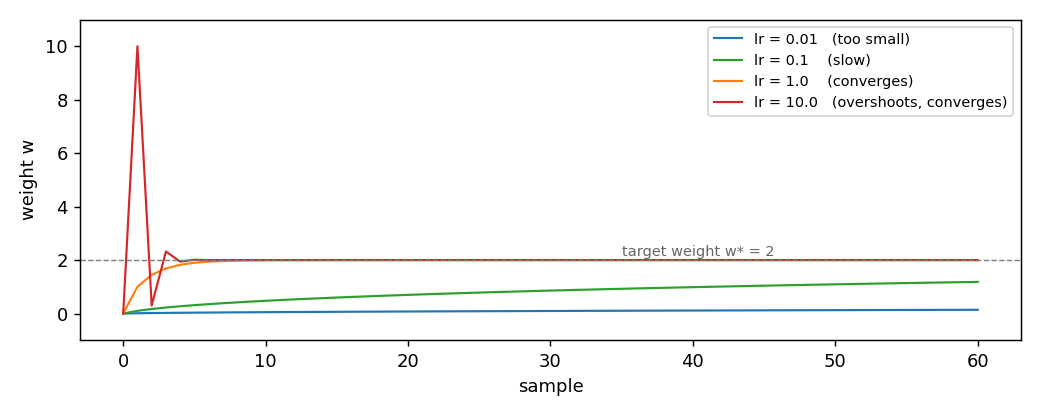
The learning rate is the only tunable parameter, and it sets the overall scale of the step. AdaGrad is more forgiving than SGD about it: a too large lr overshoots at the start, then the accumulator pulls it back. A too small lr stays slow forever, because the accumulator cannot make up for a small scalar. The figure shows four runs of the same one-feature regression, target weight w* = 2, one per lr:

lr	weight after 1 step	after 10	after 30	after 60
0.01	0.0100	0.0500	0.0950	0.1391
0.1	0.1000	0.4760	0.8579	1.1830
1.0	1.0000	1.9938	2.0000	2.0000
10.0	10.0000	2.0000	2.0000	2.0000

With lr = 10.0 the first step jumps to w = 10, well past the target. The accumulator catches it: from the second step onwards the step is small enough that the weight comes back to 2 within ten samples. With lr = 1.0 the trajectory is monotone and reaches the target around sample 30. With lr = 0.01 the model barely moves.

The lesson is that AdaGrad is robust to a large lr, but not to a small one. The default lr = 0.1 is a safe starting point; a larger value is worth trying when the data scale is unclear.

4. On a real arm

A SyntheticArm from a real Panda URDF gives q, qd, and tau at 50 Hz. The linear model learns the torque of joint 0 as a function of its velocity, one sample at a time. AdaGrad is the optimizer:

from pathlib import Path
import numpy as np
from dense_armor.utility.datasets import SyntheticArm
from dense_armor.utility.linear.glm import LinearRegression
from dense_armor.utility.optim import AdaGrad

ds = SyntheticArm(Path("test/fixtures/urdf/panda.urdf"),
                  period_s=1.0, rate_hz=50.0, n_cycles=2, seed=0)
reg = LinearRegression(optimizer=AdaGrad(lr=10.0), intercept=True,
                       feature_keys=["qd0"])
for sig, _ in ds.stream():
    reg.learn_one({"qd0": float(sig["qd_0"])}, float(sig["tau_0"]))
print(round(reg.predict_one({"qd0": 0.5}), 3))

-2.824

The same stream, with SGD(lr=1e-3), gives -2.158. The two values are close: on this one-feature problem AdaGrad does not have much to adapt to, because there is only one coordinate. The gain of AdaGrad appears when the stream has several features at very different scales, which is the case of the joint-torque regression across all seven joints of the Panda.

Details

References

Orabona, F. (2019). A Modern Introduction to Online Learning. Chapter 4, Section 4.2.4, pages 45-46, Algorithm 4.1 (AdaGrad). Theorem 4.32, page 46, gives the regret bound

Regret_T(u) <= sqrt(2) * sum_i D_i * sqrt(sum_t g_{t,i}^2)

for a hyperrectangle feasible set with per-coordinate diameters D_i.

The algorithm in this implementation is a variant of Algorithm 4.1, in the form proposed by McMahan and Streeter (2010). The source uses a per-coordinate step eta_{t,i} = sqrt(2) * D_i / (2 * sqrt(sum_j g_{j,i}^2)) and a projection onto the hyperrectangle; this implementation uses a single scalar lr shared by all coordinates and no projection. Theorem 4.32 bounds the source algorithm, not this variant.

Choices stated explicitly

• Scalar learning rate. Algorithm 4.1 uses a per-coordinate step that depends on the domain diameter D_i. This implementation takes a single lr at construction and keeps the adaptation only in the accumulator G. The variant is what dense_armor.utility.optim.AdaGrad(lr) promises in its signature, and it matches the form that has become standard in machine learning.
• No projection. The source assumes a hyperrectangle feasible set and a projection step. This implementation takes V = R^d, so the projection is the identity.
• Numerical guard eps. The source skips the update on coordinates where g_{t,i} = 0. This implementation keeps a small eps = 1e-8 in the denominator, which is equivalent in practice and simpler in the pure form.
• Accumulator grows forever. G_t is a running sum, not a running average. It never decreases. On a stationary problem that is fine; on a stream whose scale changes, AdaGrad reacts slowly, because old energy keeps pulling the step size down.

Measured cost

On one CPU thread, a LinearRegression with two features, predict_one plus learn_one per sample, median of 1000 samples after a warm-up of 200: 0.0178 ms per sample, about 25 percent more than SGD. The extra work is the accumulator update and the per-coordinate division.

Development diary

The regret bound was added after the docstring review of the task. The first version of the docstring claimed that Theorem 4.32 still bounds this variant of AdaGrad; that was wrong, and it was corrected in the same commit that added this page. The figures were regenerated for this page with the learning rates 0.01, 0.1, 1.0, 10.0. An earlier attempt used 1e-3 on the SyntheticArm stream and the model did not learn anything; lr = 10.0 was chosen after measuring the prediction at every value of the grid from 0.01 to 100.0.