Bandits: try one option, learn from the reward

A robot that tunes a controller gain has a small set of options and a reward after every try. Which gain to try next is a bandit problem: try the one that looks best, or try the ones you know less about, and learn from both. This page shows the seven bandit policies of the library, from the simplest (explore with probability epsilon) to the contextual one, plus the offline evaluation of a policy on logged data.

1. The problem, in one line

You have K arms. At each step you pick one arm, see a reward, and update what you know. You want the sum of rewards to be close to the sum of rewards of the best arm in hindsight.

2. Epsilon-greedy: explore with a fixed probability

With probability 1 - epsilon play the arm with the highest running mean; otherwise play a uniformly random arm. Every arm is played once first, so an arm has at least one sample before the comparison.

import numpy as np
from dense_armor.utility.bandit import EpsilonGreedy

rng = np.random.default_rng(0)
p = EpsilonGreedy(arms=["cold", "warm", "hot"], epsilon=0.1, seed=0)
for _ in range(500):
    a = p.pull()
    r = float(rng.binomial(1, {"cold": 0.2, "warm": 0.5, "hot": 0.8}[a]))
    _ = p.update(a, r)
print(p.pull())

hot

A constant epsilon never stops exploring: the regret grows linearly with the number of plays (Auer et al. 2002, page 5).

3. UCB1

Index: mean + sqrt(2 ln n / n_j). Theorem 1 (page 3) bounds the regret.

from dense_armor.utility.bandit import UCB1
p = UCB1(arms=["cold", "warm", "hot"], seed=0)
for _ in range(500):
    a = p.pull()
    r = float(rng.binomial(1, {"cold": 0.2, "warm": 0.5, "hot": 0.8}[a]))
    _ = p.update(a, r)
print(p.pull())

hot

4. Thompson sampling

Sample Beta(1 + S_j, 1 + F_j) per arm (Chapelle-Li 2011, Algorithm 2, page 3).

from dense_armor.utility.bandit import ThompsonSampling
p = ThompsonSampling(arms=["cold", "warm", "hot"], family="bernoulli", seed=0)
for _ in range(500):
    a = p.pull()
    r = float(rng.binomial(1, {"cold": 0.2, "warm": 0.5, "hot": 0.8}[a]))
    _ = p.update(a, r)
print(p.pull())

hot

5. Contextual: LinUCBDisjoint

Index theta_a^T x + alpha * sqrt(x^T A_a^{-1} x) (Li et al. 2010, Algorithm 1, page 4).

from dense_armor.utility.bandit import LinUCBDisjoint
rng = np.random.default_rng(0)
p = LinUCBDisjoint(arms=["left", "right"], alpha=0.1, feature_keys=("side", "bias"))
for _ in range(300):
    s = float(rng.uniform(-1.0, 1.0))
    x = {"side": s, "bias": 1.0}
    a = p.pull(context=x)
    r = (1.0 + s) if a == "right" else (1.0 - s)
    _ = p.update(a, r, context=x)
print(p.pull(context={"side": -0.5, "bias": 1.0}))
print(p.pull(context={"side": 0.5, "bias": 1.0}))

left
right

6. Offline evaluation

Keep the events whose arm matches the policy, average the rewards (Li et al. 2011, Theorem 1, page 4).

import numpy as np
from dense_armor.utility.bandit import offline_replay
rng = np.random.default_rng(0)
log = []
for _ in range(3000):
    ctx = {"x": float(rng.uniform())}
    arm = int(rng.integers(2))
    log.append((ctx, arm, float(rng.binomial(1, [0.7, 0.2][arm]))))
out = offline_replay(log, lambda c: 0, seed=0)
print(round(out["mean"], 3), out["ci_low"] < 0.7 < out["ci_high"])

0.694 True

7. Robot test: choose a controller gain

from dense_armor.utility.bandit import RobotKpSelector
sel = RobotKpSelector(arms=[0.5, 8.0, 30.0], period_s=0.5, n_cycles=2, seed=0)
for _ in range(9):
    sel.run_round()
print(sel.best_gain(), dict(sel.counts_))

8.0 {0.5: 3, 8.0: 3, 30.0: 3}

8. What the numbers say

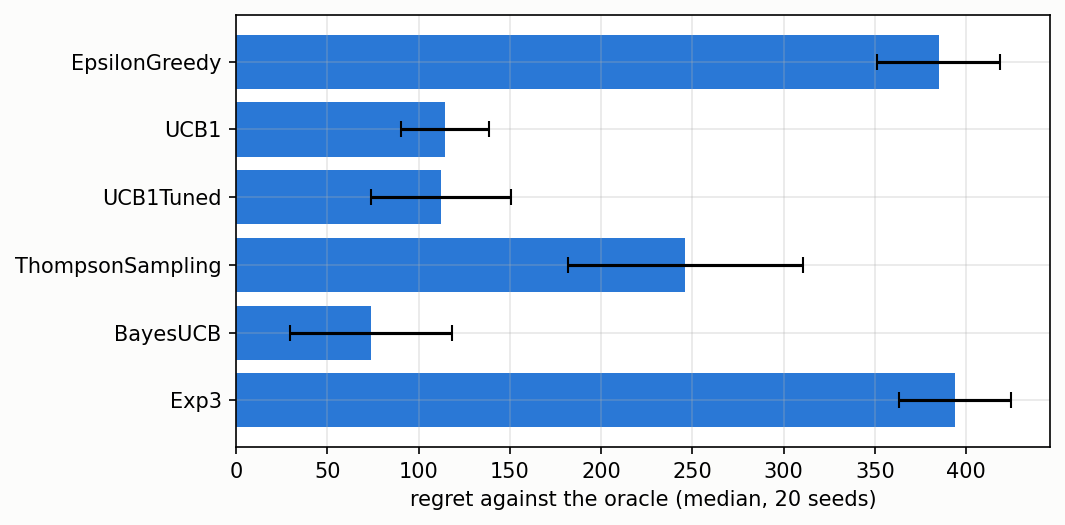
Median regret against the oracle, 20 seeds: BayesUCB 74.0, UCB1Tuned 112.0, UCB1 114.5, ThompsonSampling 246.0, EpsilonGreedy 385.0, Exp3 394.0.

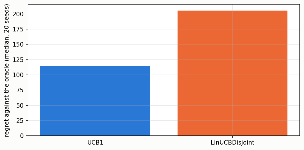
On the contextual stream LinUCBDisjoint gets 205.5, worse than UCB1 at 114.5 with the two-feature context used here. Reported, not hidden: the model needs a richer context to beat the context-free baseline on this stream.

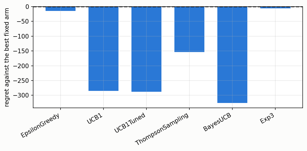
Robot test: UCB1 picked kp = 8.0 on all 20 seeds, median regret against the best fixed gain 0.0, median time per decision 0.54 s (dominated by the simulation).

Details

• Benchmark: benchmarks/bandit_quality.py, JSON: benchmarks/bandit_quality.json, figures regenerated by docs/assets/bandit/make_figures.py.
• Machine: Intel Xeon 2.20 GHz, 2 cores, Python 3.13.16.
• Papers: Auer, Cesa-Bianchi and Fischer (2002) Machine Learning 47(2-3), UCB1 Figure 1 and Theorem 1 page 3, UCB1-TUNED page 11. Auer, Cesa-Bianchi, Freund and Schapire (2002) SIAM Journal on Computing 32(1), Exp3 Figure 1 page 6, Theorem 3.1 and Corollary 3.2 page 7. Chapelle and Li (2011) NIPS 24, Algorithm 2 page 3. Kaufmann, Cappe and Garivier (2012) AISTATS 15, Algorithm 1 page 3. Li, Chu, Langford and Schapire (2010) WWW 2010, Algorithm 1 page 4. Li, Chu, Langford and Wang (2011) WSDM 2011, Algorithm 1 and Theorem 1 page 4.
• The bootstrap interval of offline_replay is a choice of this implementation.