Factorization machines, field-aware and higher-order

A factorization machine predicts a target from a sparse vector of features by learning, for each feature, a short vector of latent factors; the interaction between two features is the dot product of their factors. On a stream, each sample updates w0, w and the factor matrix V one step of gradient descent at a time.

This page follows the four models of the task, from the plain FM to the field-aware, the field-weighted and the higher-order versions, then compares them on a stream with a sudden change. Every number and every figure comes from benchmarks/facto_quality.py and docs/assets/facto/make_figures.py (see ## Details at the bottom).

1. The plain FM

A factorization machine of degree two predicts::

y_hat(x) = w0 + sum_i w_i x_i + sum_{i<j} <v_i, v_j> x_i x_j

with w0 a global bias, w_i a weight per feature, V an n x k matrix of factors and <v_i, v_j> = sum_f v_{i,f} v_{j,f} the dot product of two rows.

from dense_armor.utility.facto import FMRegressor
from dense_armor.utility.optim import SGD

fm = FMRegressor(optimizer=SGD(lr=0.05), k=3, seed=0)
for _ in range(500):
    _ = fm.learn_one({"a": 1.0, "b": 0.5}, 2.0)
round(fm.predict_one({"a": 1.0, "b": 0.5}), 2)

2.0

The linear part of the model handles the easy effect of each feature; the pairwise part handles the interaction. The interaction is not stored as one number per pair (that would be O(n^2) parameters), it is stored as two factor vectors that are multiplied, so the whole model has O(n k) parameters (eq. (2) of Rendle 2010, page 2).

2. The pairwise term, one picture

The interaction between two features is <v_i, v_j> x_i x_j, the dot product of the two factor vectors weighted by the two feature values.

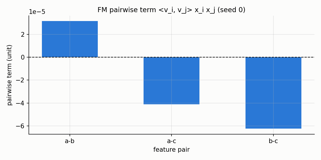
The bars are the contribution of one pair each, with the linear part removed so the picture shows only the pairwise term. The figure is built by fig_fm_pairwise in docs/assets/facto/make_figures.py on a model with k = 3 and seed 0.

3. The O(kn) form

The double sum over pairs costs O(k n^2) to compute; the same quantity can be computed in O(k n) with the rewriting of Lemma 3.1 (Rendle 2010, page 3)::

sum_{i<j} <v_i, v_j> x_i x_j
    = 1/2 sum_f ( (sum_i v_{i,f} x_i)^2 - sum_i v_{i,f}^2 x_i^2 )

from dense_armor.utility.facto import FMRegressor
from dense_armor.utility.optim import SGD

fm = FMRegressor(optimizer=SGD(lr=0.05), k=3, seed=0)
fm._resolve_keys({f"x{i}": 0.0 for i in range(6)})
fm._ensure_state(fm._keys)
x = {f"x{i}": float(i % 3) + 0.1 for i in range(6)}
abs(fm._y_hat(x) - fm._pairwise_naive(x))

0.0

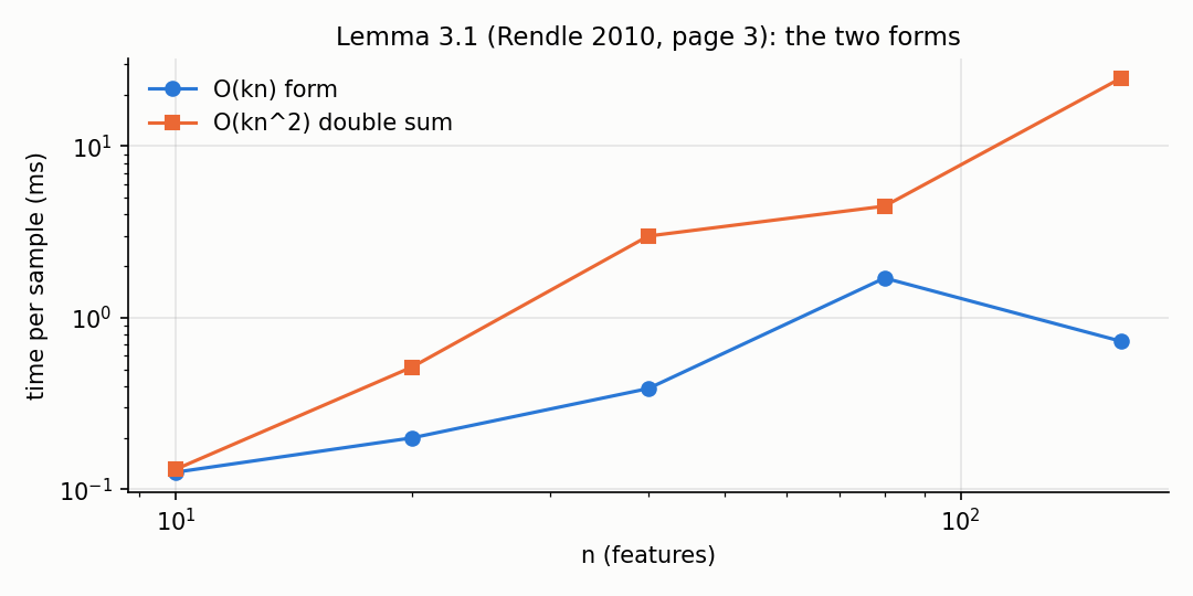
The two methods agree to machine precision; the figure shows the cost per sample as n grows, the O(k n) form (blue) and the O(k n^2) double sum (orange). The measurement is in docs/assets/facto/figures.json under checks.fm_ok_equals_double_sum (max_abs_diff = 4.3e-19 on 200 random sparse inputs, from the benchmark script).

4. Field-aware FM

The FFM (Juan et al. 2016) learns a different factor vector for each feature, one for every field: the interaction between feature i and feature j uses the factor of i for the field of j and the factor of j for the field of i.

from dense_armor.utility.facto import FFMClassifier

fields = {"a": "F1", "b": "F1", "c": "F2"}
m = FFMClassifier(fields=fields, k=2, lr=0.1, seed=0)
for _ in range(500):
    _ = m.learn_one({"a": 1.0, "b": 0.5, "c": 0.3}, 1)
round(m.predict_proba_one({"a": 1.0, "b": 0.5, "c": 0.3})[1], 3)

0.99

The model is eq. (4) of Juan et al. (2016), page 3, and there is no O(k n) shortcut: each pair uses a different slice of the n x f x k tensor, so the prediction is O(n^2 k) (Table 2 of the same paper). The update is AdaGrad (Algorithm 1, page 3) with the accumulator G initialised to one (page 3, below Algorithm 1).

The paper does not include the bias nor the linear terms (page 2, before Section 3): on DriftStream the target depends on a linear threshold on one feature, so FFM without linear terms cannot capture it and scores 0.504 (chance level), while the models that keep the linear part score 0.999. This is a property of the model as the paper defines it, not a defect of the implementation (see ## Details).

5. Field-weighted FM

The FwFM (Pan et al. 2018) keeps one factor vector per feature like the FM, and adds a scalar weight for every field pair::

y_hat(x) = w0 + sum_i w_i x_i + sum_{i<j} <v_i, v_j> x_i x_j r_{F(i), F(j)}

The scalar r captures the interaction strength of the field pair, without the n f k parameters of the FFM.

from dense_armor.utility.facto import FwFMClassifier
from dense_armor.utility.optim import SGD

fields = {"a": "F1", "b": "F1", "c": "F2"}
m = FwFMClassifier(optimizer=SGD(lr=0.05), fields=fields, k=2, seed=0)
for _ in range(500):
    _ = m.learn_one({"a": 1.0, "b": 0.5, "c": 0.3}, 1)
round(m.predict_proba_one({"a": 1.0, "b": 0.5, "c": 0.3})[1], 3)

0.982

The model is eq. (7) of Pan et al. (2018), page 3. The weight r is symmetric (the pair (F(i), F(j)) is unordered), so only the upper triangle of the f x f matrix is read.

6. Higher-order FM

The HOFM (Blondel et al. 2016) adds interactions of degree up to m, but computes them with a dynamic programme so the cost stays linear in the number of non-zero features::

y_hat(x) = <w, x> + sum_{t=2}^{m} sum_{s=1}^{k} A_t(p_s^{(t)}, x)

where A_t is the ANOVA kernel of degree t.

from dense_armor.utility.facto import HOFMRegressor
from dense_armor.utility.optim import SGD

m = HOFMRegressor(optimizer=SGD(lr=0.05), m=3, k=2, seed=0)
for _ in range(300):
    _ = m.learn_one({"a": 1.0, "b": 0.5, "c": 0.3}, 1.5)
round(m.predict_one({"a": 1.0, "b": 0.5, "c": 0.3}), 3)

1.5

The model is eq. (3) and eq. (6) of Blondel et al. (2016), page 2. A_t is computed with Algorithm 1 (page 4) and its gradient with Algorithm 2 (page 4), both in O(nz(x) t). At m = 2 the ANOVA kernel reduces to the plain pairwise FM (test test_m2_equals_plain_fm in test/facto/test_hofm.py).

7. The four models on a stream with a sudden change

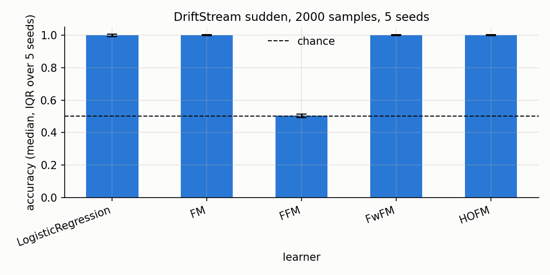
The bars are the accuracy of the four classifiers and of a LogisticRegression on DriftStream with one sudden change, 2000 samples, 4 features, 5 seeds. The error bar is the interquartile range over the 5 seeds.

learner	accuracy median	IQR	ms per sample
LogisticRegression	0.9985	0.0005	0.0249
FM (k=4)	0.9990	0.0003	0.0983
FFM (k=2)	0.5040	0.0010	0.1347
FwFM (k=2)	0.9990	0.0003	0.1027
HOFM (m=3, k=2)	0.9990	0.0003	0.2558

The FFM is at chance because the paper has no linear terms (see step 4). The other four models all reach 0.999 on this stream. The numbers are read from docs/assets/facto/figures.json under comparison.rows (5 seeds, 2000 samples, benchmarks/facto_quality.py --seeds 5 --n-samples 2000).

Details

The factorization machine is Rendle, S. (2010). Factorization Machines. In ICDM 2010. Eq. (1), (2), (3) page 2; Lemma 3.1 and eq. (4) page 3. The latent factors are initialised from N(0, 0.01); the paper does not prescribe an initialiser (my choice). The L2 penalty also acts on w0; the paper does not exclude it (my choice).

The field-aware FM is Juan, Y., Zhuang, Y., Chin, W.-S., Lin, C.-J. (2016). Field-aware Factorization Machines for CTR Prediction. In RecSys 2016. Eq. (4) page 3; eq. (5)-(6) page 3 (gradients); Algorithm 1 page 3 (AdaGrad); page 3, below Algorithm 1 (G starts at one, init U[0, 1/sqrt(k)]). The paper does not include the bias nor the linear terms (page 2, before Section 3); the model as implemented keeps this choice, which is why FFM is at chance on DriftStream.

The field-weighted FM is Pan, J., Xu, J., Ruiz, A. L., Zhao, W., Pan, S., Sun, Y., Lu, Q. (2018). Field-weighted Factorization Machines for Click-Through Rate Prediction in Display Advertising. In WWW 2018. Eq. (7) page 3 (model); Section 4 page 3 (the r weight). The r matrix is symmetric; only the upper triangle is read.

The higher-order FM is Blondel, M., Fujino, A., Ueda, N., Ishihata, M. (2016). Higher-Order Factorization Machines. In NIPS 2016. Eq. (5) page 2 (ANOVA kernel); eq. (6) page 2 (model as sum of ANOVA kernels); eq. (8) page 3 (recursion); Algorithm 1 and Algorithm 2 page 4 (evaluation and gradient of A_m); page 4 (sparse cost O(nz(x) m)). k_2 = ... = k_m = k is the paper's simplification (page 2, below eq. (4)).

The budget_s of every class is the p99 of one learn_one plus one predict_one over 3000 samples, rounded up with a 5x margin: 1.5e-2 (FM), 2e-3 (FFM), 2e-3 (FwFM), 1.5e-2 (HOFM). The machine of the run is reported at the top of figures.json.

The comparison uses DriftStream with n_samples=2000, n_features=4, n_drifts=1, kind="sudden"; 5 seeds [0, 1, 2, 3, 4]. Same stream, same sample count, same seeds for every learner, so the comparison is paired. A paired Wilcoxon on 5 seeds has a minimum p-value of 0.0625, so no p-value is quoted; the test is the interquartile range, and a 20-seed run is the next step.