Metrics and evaluation
A robot that keeps learning needs to know whether it is learning well. These tools keep a small running score that is updated every time a new reading arrives and its answer can be compared with what really happened.
What this is
A robot that learns while it works needs a way to tell whether it is learning well. You cannot stop it, collect a test set and score it at the end: the data never ends and the world changes under it. The answer is to score it as it goes: every time a new sample arrives, compare what the model predicted with what really happened, and keep a small running summary.
This page shows those running summaries (the metrics), the protocol that feeds them (predict first, then learn), and the metrics made for events on a robot: how fast a fault is caught and how often the alarm rings for nothing.
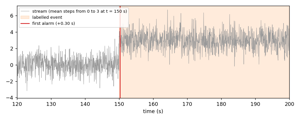
The figure is the case this page builds towards: a signal sampled at 20 Hz changes at t = 150 s, a drift detector raises its first alarm 0.30 s later, and the metrics turn that into numbers: delay, missed events, false alarms per hour.
1. A metric, one pair at a time
A metric reads one pair (y_true, y_pred) with update and answers get() at any moment.
from dense_armor.utility.metrics import Accuracy

m = Accuracy()
for y, p in [(0, 0), (1, 1), (0, 1), (1, 1)]:
    m.update(y, p)
print(m.get(), m.n)
Three of the four predictions are right, so the accuracy is 3/4 = 0.75. The metric keeps two running sums (hits and total), not the list of pairs, so its memory stays the same after a million samples. Every metric on this page has the same members:
update(y_true, y_pred, t=None, w=1.0)adds a pair, with an optional timestamp and weight;revert(y_true, y_pred)removes a pair added before (used by the rolling windows of step 6);merge(other)combines two metrics computed on different parts of the stream;ncounts the pairs used,n_missingthe pairs skipped because one side wasNoneorNaN;works_with(model)tells whether the metric fits the model's role (classifier or regressor).
2. Classification: precision, recall, F1
When the model says "positive", how often is it right (precision)? Of the real positives, how many did it find (recall)? F1 is their harmonic mean.
from dense_armor.utility.metrics import F1, Precision, Recall

y = [1, 0, 1, 1, 0, 1]
p = [1, 1, 1, 0, 0, 1]
ms = [Precision(positive=1), Recall(positive=1), F1(positive=1), F1(average="macro")]
for a, b in zip(y, p):
    for m in ms:
        m.update(a, b)
print([round(m.get(), 3) for m in ms])
Count by hand for class 1: true positives TP = 3 (positions 0, 2, 5), one false positive FP (position 1), one false negative FN (position 3).
$$P = \frac{TP}{TP + FP} = \frac{3}{4}, \qquad R = \frac{TP}{TP + FN} = \frac{3}{4}, \qquad F_1 = \frac{2PR}{P + R} = 0.75.$$
average="macro" computes F1 for every class and takes the plain mean: class 0 has TP = 1,
FP = 1, FN = 1, so F1 = 0.5, and the macro F1 is (0.75 + 0.5) / 2 = 0.625. "micro" pools the
counts of all classes, "weighted" weights each class by how often it occurs; FBeta(beta=2)
weights recall more than precision.
3. Agreement beyond chance and probabilities
Accuracy can look good by chance when one class is common. Cohen's kappa subtracts the agreement expected by chance.
from dense_armor.utility.metrics import CohenKappa

m = CohenKappa()
for a, b in zip([1, 0, 1, 1, 0, 1], [1, 1, 1, 0, 0, 1]):
    m.update(a, b)
print(round(m.get(), 3))
$$\kappa = \frac{p_o - p_e}{1 - p_e}$$
where $p_o$ is the observed agreement (4 of 6) and $p_e$ the agreement two independent guessers with the same label frequencies would reach: both say 1 four times out of six and 0 twice, so $p_e = (4 \cdot 4 + 2 \cdot 2)/36 = 0.556$ and $\kappa = (0.667 - 0.556)/(1 - 0.556) = 0.25$.
When the model gives a probability instead of a label, score the probability itself.
from dense_armor.utility.metrics import BrierScore, LogLoss

ll, br = LogLoss(), BrierScore()
for y, p in [(1, 0.9), (0, 0.2), (1, 0.6)]:
    ll.update(y, p)
    br.update(y, p)
print(round(ll.get(), 4), round(br.get(), 4))
The log-loss is the mean of $-\ln p$ given to what happened: $-(\ln 0.9 + \ln 0.8 + \ln 0.6)/3 = 0.2798$. The Brier score is the mean squared distance between probability and outcome: $(0.1^2 + 0.2^2 + 0.4^2)/3 = 0.07$. Both are lower for better forecasts.
4. Regression on a joint
A regressor predicts a number, for example the torque a joint needs at a given velocity. Here a recursive least-squares model learns $\tau = 2\,\dot q$ from noisy samples, and three metrics score it before each update.
import numpy as np
from dense_armor.utility.learn.online_dynamics import RecursiveLeastSquares
from dense_armor.utility.metrics import MeanAbsoluteError, R2Score, RootMeanSquaredError

rng = np.random.default_rng(0)
rls, ms = RecursiveLeastSquares(), [MeanAbsoluteError(), RootMeanSquaredError(), R2Score()]
for qd in rng.normal(0, 1, 500):
    tau = 2.0 * qd + rng.normal(0, 0.1)
    for m in ms:
        m.update(tau, rls.predict_one({"qd": qd}))
    rls.learn_one({"qd": qd}, tau)
print([round(m.get(), 3) for m in ms])
The MAE is the mean of $|\tau - \hat\tau|$, the RMSE the square root of the mean of $(\tau - \hat\tau)^2$, both in the units of the torque. They sit near the noise level: for noise with standard deviation 0.1 the RMSE tends to 0.1 and the MAE to $0.1\sqrt{2/\pi} = 0.080$. $R^2 = 1 - \sum(\tau - \hat\tau)^2 / \sum(\tau - \bar\tau)^2$ compares the model with always predicting the mean: 0.998 means the model explains almost all the variation.
A robot arm has several joints. Pass the vector and the metric reports each joint and the mean.
from dense_armor.utility.metrics import MeanAbsoluteError

m = MeanAbsoluteError()
m.update([1.0, 2.0], [1.5, 2.5])
m.update([2.0, 4.0], [2.5, 3.0])
print(m.get())
Joint 0 is off by 0.5 both times; joint 1 by 0.5 and then 1.0, mean 0.75.
5. Scoring the uncertainty
A prediction with an interval is useful only if the interval is honest. Two numbers check it: how often the truth falls inside (coverage) and how wide the interval is (width).
import numpy as np
from dense_armor.roles import AdaptiveConformalRegressor
from dense_armor.utility.learn.online_dynamics import RecursiveLeastSquares
from dense_armor.utility.metrics import IntervalCoverage, MeanIntervalWidth

rng = np.random.default_rng(0)
acr, cov, wid = AdaptiveConformalRegressor(RecursiveLeastSquares(), alpha=0.1), IntervalCoverage(), MeanIntervalWidth()
for qd in rng.normal(0, 1, 2000):
    x, tau = {"qd": qd}, 2.0 * qd + rng.normal(0, 0.1)
    cov.update(tau, acr.predict_interval(x))
    wid.update(tau, acr.predict_interval(x))
    acr.learn_one(x, tau)
print(round(cov.get(), 3), round(wid.get(), 3))
The interval was asked for 90 % coverage (alpha=0.1) and covers 90 % of the torques. Its mean
width 0.34 is close to the narrowest honest 90 % interval for Gaussian noise of standard
deviation 0.1, which is $2 \cdot 1.645 \cdot 0.1 = 0.33$.
When the prediction is a mean and a variance, the Gaussian negative log-likelihood scores both at once.
from dense_armor.roles import Estimate
from dense_armor.utility.metrics import GaussianNLL

m = GaussianNLL()
m.update(0.1, Estimate(mean=0.0, var=0.01))
print(round(m.get(), 4))
$$\mathrm{NLL} = \tfrac12 \ln(2\pi v) + \frac{(y - \mu)^2}{2v} = \tfrac12 \ln(0.0628) + \tfrac12 = -0.8836.$$
A variance that is too small makes the second term explode; one that is too large makes the first term grow. The minimum is at the true spread.
6. Windows: only the recent past
A robot changes over time; the accuracy of last week says little about now. Rolling keeps a
metric over the last window samples, or the last window_s seconds.
from dense_armor.utility.metrics import Accuracy, Rolling

m = Rolling(Accuracy(), window_s=0.05)
for i in range(20):
    m.update(1 if i < 17 else 0, 1, t=i * 0.01)
print(m.count, m.get())
At 100 Hz a window of 0.05 s holds 5 samples: the window keeps the samples with
$t_\text{now} - t < 0.05$. The last three predictions are wrong, so the accuracy over the
window is 2/5. The window uses the timestamps, not the sample count, so a dropped sample does
not stretch it. Any metric with revert can be rolled.
The ROC-AUC is the probability that a random positive gets a higher score than a random
negative. RollingAUC computes it exactly on the last window pairs.
import numpy as np
from dense_armor.utility.metrics import RollingAUC

rng = np.random.default_rng(0)
m = RollingAUC(window=200)
for _ in range(1000):
    y = int(rng.random() < 0.3)
    m.update(y, y + rng.normal(0, 1.0))
print(round(m.get(), 3))
$$\mathrm{AUC} = \frac{1}{n_+ n_-}\sum_{i \in +}\sum_{j \in -} \begin{cases} 1 & s_i > s_j \ \tfrac12 & s_i = s_j \ 0 & \text{otherwise} \end{cases}$$
Here positives score one unit higher than negatives with unit noise, so the long-run value is $\Phi(1/\sqrt2) = 0.760$; a window of 200 pairs gives 0.712.
7. Predict, then learn
progressive_val_score runs the protocol for you: for each sample the model predicts, the
metric scores, then the model learns. Labels often arrive late (a technician confirms a fault at
the end of the shift); with delay the model learns each label only when it arrives.
import numpy as np
from dense_armor.utility.evaluate import progressive_val_score
from dense_armor.utility.learn.online_classifiers import OnlineGaussianNB
from dense_armor.utility.metrics import Accuracy, Rolling

rng = np.random.default_rng(0)
qd = rng.normal(0, 1, 2000)
y = np.abs(qd) > np.where(np.arange(2000) < 1000, 0.5, 1.5)
s = [({"qd": a}, int(b)) for a, b in zip(qd, y)]
for d in (None, 300):
    m, tr = progressive_val_score(s, OnlineGaussianNB(), Rolling(Accuracy(), window=200), delay=d, every=200)
    print(d, [round(r, 2) for r in tr])
None [0.91, 0.94, 0.95, 0.95, 0.92, 0.54, 0.66, 0.76, 0.84, 0.84]
300 [0.0, 0.0, 0.0, 0.89, 0.95, 0.92, 0.71, 0.38, 0.59, 0.7]
The task is "is the joint moving fast?", and at sample 1000 the meaning of "fast" changes from
$|\dot q| > 0.5$ to $|\dot q| > 1.5$. With labels on time the rolling accuracy drops to 0.54 and
recovers to 0.84. With labels 300 samples late the drop comes later and goes deeper (0.38),
because the model keeps answering with the old rule until the new labels reach it. For delay=300 the first
three values are 0.0 because no label has arrived yet and nothing has been scored. every=200
returns the trace of the metric.
For metrics that need a probability, progressive_val_proba_score uses predict_proba_one.
import numpy as np
from dense_armor.utility.evaluate import progressive_val_proba_score
from dense_armor.utility.learn.online_classifiers import OnlineGaussianNB
from dense_armor.utility.metrics import LogLoss

rng = np.random.default_rng(0)
s = [({"qd": v}, int(abs(v) > 0.5)) for v in rng.normal(0, 1, 2000)]
m, tr = progressive_val_proba_score(s, OnlineGaussianNB(), LogLoss(), every=500)
print([round(v, 3) for v in tr])
The log-loss falls as the model sees more samples.
8. Choosing a model on the stream
best_of runs several models on the same stream with the same protocol and tells which one is
ahead.
import numpy as np
from dense_armor.utility.evaluate import best_of
from dense_armor.utility.learn.online_classifiers import OnlineGaussianNB, OnlineSoftmaxRegression
from dense_armor.utility.metrics import Accuracy

rng = np.random.default_rng(0)
s = [({"qd": v}, int(abs(v) > 0.5)) for v in rng.normal(0, 1, 2000)]
sel = best_of([OnlineGaussianNB(), OnlineSoftmaxRegression()], Accuracy, stream=s)
print([round(v, 3) for v in sel.scores()], sel.current_best())
"Fast in either direction" is not a straight cut on $\dot q$, so a linear softmax model cannot
learn it (0.621), while the Gaussian model, which learns a different spread per class, can
(0.941). current_best() returns the index 0 and best_model() the model itself. The second
argument is the metric class: each model gets its own fresh metric.
9. Events: delay and false alarms
A fault is not one sample: it lasts. EventMetrics takes the labelled event windows, then the
alarm times, and answers the two questions a robot operator asks: how late was the alarm, and
how often does it ring for nothing?
from dense_armor.utility.metrics import EventMetrics

m = EventMetrics([(10.0, 20.0), (40.0, 45.0)], dt=0.5, normal_time_s=3600.0)
for t in (5.0, 12.0, 12.5, 30.0):
    m.add_alarm(t)
print(m.detection_delays_s(), m.missed_events(), m.false_alarms(), m.false_alarms_per_hour())
The first event starts at 10 s and the first alarm inside it is at 12 s: delay 2 s. The second
event has no alarm: missed. The alarms at 5 s and 30 s are outside every event: two false
alarms over one hour of normal operation, 2 per hour. dt is the sample period, used in step
10 to count the points of a window.
10. How much of the event was caught
Tatbul et al. (2018) extend precision and recall to ranges. The recall of one real event mixes two rewards:
$$\mathrm{Recall}(R_i, P) = \alpha \cdot \mathrm{Existence}(R_i, P) + (1 - \alpha) \cdot \mathrm{Overlap}(R_i, P) \qquad \text{(Eq. 4)}$$
The existence reward is 1 if any alarm falls inside the event (Eq. 5). The overlap reward (Eq. 6) adds up a weight $\delta(i)$ for every point $i$ of the event that the alarms cover, divided by the sum of all the weights, and is shrunk by a cardinality factor when the event is split across several alarm ranges (Eq. 7). The weights are the positional bias of their Figure 2b: flat ($\delta = 1$), front ($\delta = L - i + 1$, early points count more), back ($\delta = i$), middle. Precision (Eq. 9) uses the same overlap reward, with flat bias.
from dense_armor.utility.metrics import EventMetrics

for bias in ("front", "back"):
    m = EventMetrics([(0.0, 9.0)], positional_bias=bias, threshold_window=1.0)
    for t in (0.0, 1.0, 2.0):
        m.add_alarm(t)
    print(bias, round(m.range_precision(), 3), round(m.range_recall(), 3), round(m.range_f1(), 3))
The event has 10 points (0 to 9 s at dt=1.0); the three alarms, merged into one range by
threshold_window=1.0, cover the first three. With front bias the weights are 10, 9, …, 1
(sum 55) and the covered ones add up to 10 + 9 + 8 = 27: recall 27/55 = 0.491. With back bias
they are 1 + 2 + 3 = 6: recall 6/55 = 0.109. Precision is 1.0 in both cases because every alarm
point lies inside the event. For a robot, front bias says "catching the start of a fault is what
matters".
11. One score for early detection: NAB
The Numenta Anomaly Benchmark (Lavin and Ahmad 2015) gives each detection a weight that depends on where it falls.
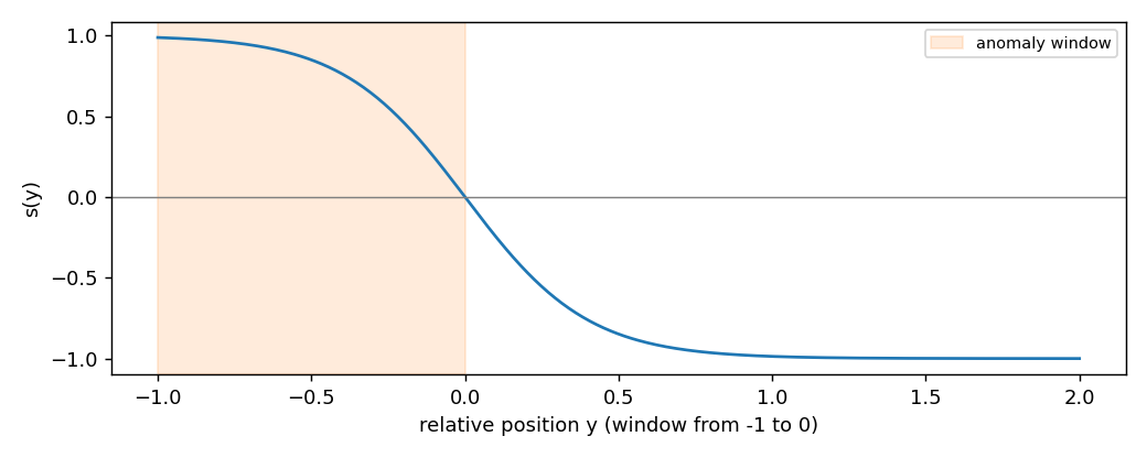
$$s(y) = \frac{2}{1 + e^{5y}} - 1$$
where $y$ is the position relative to the window: $-1$ at its start, $0$ at its end, positive after it. The earliest detection in a window earns $A_{TP}\,s(y)$; a missed window costs $A_{FN}$; an alarm outside every window costs $|A_{FP}|\,s(y)$ measured after the preceding window, or $-|A_{FP}|$ if no window precedes it. The total is normalised so that a perfect detector scores 100 and a detector that never fires scores 0 (Eq. 4).
from dense_armor.utility.metrics import EventMetrics

for alarms in ([0.0], [9.0], [9.0, 14.5], []):
    m = EventMetrics([(0.0, 10.0)])
    for t in alarms:
        m.add_alarm(t)
    print(alarms, round(m.nab_score(), 2))
A detection at 9 s in a window from 0 to 10 s has $y = -0.1$ and earns $s = 0.245$; normalised
between the null detector ($-1$) and the perfect one ($s(-1) = 0.987$) it gives
$100 \cdot 1.245 / 1.987 = 62.67$. The extra alarm at 14.5 s is 0.45 windows after the end:
$s = -0.809$, times $|A_{FP}| = 0.11$, which lowers the score to 58.18. The default weights are
the paper's standard profile ($A_{TP} = 1$, $A_{FP} = -0.11$, $A_{FN} = -1$); pass a_tp,
a_fp, a_fn to change them.
12. A real detector on a stream
evaluate_events runs a detector over (t, x) pairs and returns everything at once. This is
the case of the figure at the top.
import numpy as np
from dense_armor.utility.drift.detector import CUSUMDriftDetector
from dense_armor.utility.evaluate import evaluate_events

rng = np.random.default_rng(1)
x = np.concatenate([rng.normal(0, 1, 3000), rng.normal(3, 1, 1000)])
det = CUSUMDriftDetector(reference="fixed", radius=76, ref_mult=10, k=0.5, h=20.0)
s = [(i / 20, v) for i, v in enumerate(x)]
r = evaluate_events(s, det, [(150.0, 199.95)], dt=0.05, normal_time_s=150.0)
print(round(r["detection_delays_s"][0], 2), r["missed"], r["false_alarms_per_hour"])
The CUSUM detector catches the step 0.30 s after it starts (6 samples at 20 Hz), misses
nothing and raises no alarm during the 150 s of normal operation. The returned dict also holds
range_precision, range_recall, range_f1 and nab_score. A drift detector is read
through update and drift_detected; an anomaly detector through score_one, learn_one and
a score_threshold attribute.
13. A warning: point-adjusted F1
Many papers score anomaly detectors with point adjustment: if one point inside a real anomaly is flagged, the whole anomaly counts as found. Kim et al. (2021) show that this rewards noise.
import numpy as np
from dense_armor.utility.metrics import F1, PointAdjustedF1

rng = np.random.default_rng(0)
y = np.zeros(2000, dtype=int)
for s in (200, 700, 1200, 1700):
    y[s:s + 100] = 1
p = (rng.random(2000) < 0.05).astype(int)
pa, f1 = PointAdjustedF1(positive=1, warn=False), F1(positive=1)
for a, b in zip(y.tolist(), p.tolist()):
    pa.update(a, b)
    f1.update(a, b)
print(round(pa.get(), 3), round(f1.get(), 3))
The "detector" flags 5 % of the samples at random. The plain F1 is 0.063, as it should be; the
point-adjusted F1 is 0.895, because each 100-sample anomaly almost surely contains one random
flag. PointAdjustedF1 is here only to compare with published numbers; it warns when read.
Report the range-based metrics of step 10 next to it.
API reference
metrics 
Online metrics for streams, robots and LLMs.
Metric 
Base class for online metrics.
Subclasses override _update, _revert, get and merge;
the base handles the validity check, the count and the timestamp.
Attributes:
| Name | Type | Description |
|---|---|---|
role_ |
Any
|
role class the metric applies to, or |
bigger_is_better |
bool
|
|
Source code in dense_armor/utility/metrics/base.py
update 
Feed one pair into the metric.
Parameters:
| Name | Type | Description | Default |
|---|---|---|---|
y_true
|
Any
|
the observed label. |
required |
y_pred
|
Any
|
the predicted label. |
required |
t
|
float | None
|
timestamp in seconds; not required by every metric. |
None
|
w
|
float
|
sample weight, default 1.0. |
1.0
|
Returns:
| Type | Description |
|---|---|
Metric
|
|
Source code in dense_armor/utility/metrics/base.py
revert 
Undo one update. Used by the rolling wrappers.
Parameters:
| Name | Type | Description | Default |
|---|---|---|---|
y_true
|
Any
|
the label that was passed to |
required |
y_pred
|
Any
|
the prediction that was passed to |
required |
w
|
float
|
the same weight used in |
1.0
|
Returns:
| Type | Description |
|---|---|
Metric
|
|
Source code in dense_armor/utility/metrics/base.py
get 
Return the current value of the metric.
Most metrics return a float. :class:ConfusionMatrix is
the one exception: it returns a nested dict
{y_true: {y_pred: count}}, which is why the return type
here is Any. Concrete subclasses refine it.
Source code in dense_armor/utility/metrics/base.py
merge 
works_with 
F1 
Bases: FBeta
F1 score: the harmonic mean of precision and recall.
A thin subclass of :class:FBeta with beta = 1.0.
Examples:
>>> from dense_armor.utility.metrics import F1
>>> m = F1(positive=1)
>>> for a, b in [(1, 1), (0, 1), (1, 1)]:
...     _ = m.update(a, b)
>>> round(m.get(), 4)
0.8
Source code in dense_armor/utility/metrics/classification.py
merge 
Combine two partial states, keeping the F1 class.
Parameters:
| Name | Type | Description | Default |
|---|---|---|---|
other
|
Metric
|
another :class: |
required |
Returns:
| Type | Description |
|---|---|
F1
|
A new :class: |
Raises:
| Type | Description |
|---|---|
TypeError
|
if |
Source code in dense_armor/utility/metrics/classification.py
Accuracy 
Bases: Metric
Fraction of samples where y_pred == y_true.
Examples:
>>> from dense_armor.utility.metrics import Accuracy
>>> m = Accuracy()
>>> for a, b in [(0, 0), (1, 1), (0, 1), (1, 1)]:
...     _ = m.update(a, b)
>>> m.get()
0.75
Source code in dense_armor/utility/metrics/classification.py
merge 
Combine two partial states.
Parameters:
| Name | Type | Description | Default |
|---|---|---|---|
other
|
Metric
|
another :class: |
required |
Returns:
| Type | Description |
|---|---|
Accuracy
|
A new :class: |
Raises:
| Type | Description |
|---|---|
TypeError
|
if |
Source code in dense_armor/utility/metrics/classification.py
BalancedAccuracy 
Bases: Metric
Mean of the per-class recall.
For binary classification with classes 0 and 1 this is
(TPR + TNR) / 2, where TNR is the recall of the negative
class. Balanced accuracy is the natural metric for imbalanced
streams, since a majority-class predictor scores 0.5.
Examples:
>>> from dense_armor.utility.metrics import BalancedAccuracy
>>> m = BalancedAccuracy()
>>> for a, b in [(0, 0), (0, 1), (1, 1), (1, 1)]:
...     _ = m.update(a, b)
>>> round(m.get(), 4)
0.75
Source code in dense_armor/utility/metrics/classification.py
merge 
Combine two partial states.
Parameters:
| Name | Type | Description | Default |
|---|---|---|---|
other
|
Metric
|
another :class: |
required |
Returns:
| Type | Description |
|---|---|
BalancedAccuracy
|
A new :class: |
Raises:
| Type | Description |
|---|---|
TypeError
|
if |
Source code in dense_armor/utility/metrics/classification.py
BrierScore 
Bases: Metric
Mean squared error of predicted probabilities.
mean((p - y)**2). The lower the better; 0.25 is the score of
a constant 0.5 forecast.
Examples:
>>> from dense_armor.utility.metrics import BrierScore
>>> m = BrierScore()
>>> for y, p in [(1, 0.9), (0, 0.1)]:
...     _ = m.update(y, p)
>>> round(m.get(), 4)
0.01
Source code in dense_armor/utility/metrics/classification.py
merge 
Combine two partial states.
Parameters:
| Name | Type | Description | Default |
|---|---|---|---|
other
|
Metric
|
another :class: |
required |
Returns:
| Type | Description |
|---|---|
BrierScore
|
A new :class: |
Raises:
| Type | Description |
|---|---|
TypeError
|
if |
Source code in dense_armor/utility/metrics/classification.py
CohenKappa 
Bases: Metric
Cohen's kappa: agreement corrected for chance.
kappa = (p_o - p_e) / (1 - p_e) where p_o is the observed
agreement and p_e is the agreement expected by chance under the
marginal label frequencies. 1.0 is perfect, 0.0 is chance,
negative is worse than chance.
References
Cohen, J. (1960). Educational and Psychological Measurement 20(1), 37-46.
Source code in dense_armor/utility/metrics/classification.py
merge 
Combine two partial states.
Parameters:
| Name | Type | Description | Default |
|---|---|---|---|
other
|
Metric
|
another :class: |
required |
Returns:
| Type | Description |
|---|---|
CohenKappa
|
A new :class: |
Raises:
| Type | Description |
|---|---|
TypeError
|
if |
Source code in dense_armor/utility/metrics/classification.py
ConfusionMatrix 
Bases: Metric
Multiclass confusion matrix.
get() returns a nested dict {y_true: {y_pred: count}}, so
this metric is the one exception to the get() -> float
convention; works_with still uses the classifier role.
Examples:
>>> from dense_armor.utility.metrics import ConfusionMatrix
>>> m = ConfusionMatrix()
>>> for a, b in [(0, 0), (0, 1), (1, 1)]:
...     _ = m.update(a, b)
>>> m.get()[0][1]
1.0
Source code in dense_armor/utility/metrics/classification.py
merge 
Combine two partial states.
Parameters:
| Name | Type | Description | Default |
|---|---|---|---|
other
|
Metric
|
another :class: |
required |
Returns:
| Type | Description |
|---|---|
ConfusionMatrix
|
A new :class: |
Raises:
| Type | Description |
|---|---|
TypeError
|
if |
Source code in dense_armor/utility/metrics/classification.py
FBeta 
Bases: _PRFBase
Weighted harmonic mean of precision and recall.
F_beta = (1 + beta**2) * P * R / (beta**2 * P + R). F1 is
the special case beta = 1. The average follows the same
conventions as :class:Precision.
Parameters:
| Name | Type | Description | Default |
|---|---|---|---|
beta
|
float
|
relative weight of recall over precision. |
1.0
|
positive
|
Any
|
the label treated as positive in |
True
|
average
|
str
|
|
'binary'
|
Examples:
>>> from dense_armor.utility.metrics import FBeta
>>> m = FBeta(beta=1.0, positive=1)
>>> for a, b in [(1, 1), (0, 1), (1, 1), (0, 0)]:
...     _ = m.update(a, b)
>>> round(m.get(), 4)
0.8
Source code in dense_armor/utility/metrics/classification.py
merge 
Combine two partial states.
Parameters:
| Name | Type | Description | Default |
|---|---|---|---|
other
|
Metric
|
another :class: |
required |
Returns:
| Type | Description |
|---|---|
FBeta
|
A new :class: |
Raises:
| Type | Description |
|---|---|
TypeError
|
if |
Source code in dense_armor/utility/metrics/classification.py
LogLoss 
Bases: Metric
Binary log-loss (cross-entropy).
-mean(y log p + (1 - y) log(1 - p)) with p the predicted
probability of the positive class. The predicted probability is
clipped to [eps, 1 - eps] to avoid log(0).
Parameters:
| Name | Type | Description | Default |
|---|---|---|---|
eps
|
float
|
clipping floor, default |
1e-15
|
Examples:
>>> from dense_armor.utility.metrics import LogLoss
>>> m = LogLoss()
>>> for y, p in [(1, 0.9), (0, 0.1)]:
...     _ = m.update(y, p)
>>> round(m.get(), 4)
0.1054
Source code in dense_armor/utility/metrics/classification.py
merge 
Combine two partial states.
Parameters:
| Name | Type | Description | Default |
|---|---|---|---|
other
|
Metric
|
another :class: |
required |
Returns:
| Type | Description |
|---|---|
LogLoss
|
A new :class: |
Raises:
| Type | Description |
|---|---|
TypeError
|
if |
Source code in dense_armor/utility/metrics/classification.py
Precision 
Bases: _PRFBase
Fraction of predicted positives that are correct.
Supports four averages: "binary" (uses positive),
"macro", "micro", "weighted".
Examples:
>>> from dense_armor.utility.metrics import Precision
>>> m = Precision(positive=1, average="binary")
>>> for a, b in [(1, 1), (0, 1), (1, 1), (0, 0)]:
...     _ = m.update(a, b)
>>> m.get()
0.6666666666666666
Source code in dense_armor/utility/metrics/classification.py
merge 
Combine two partial states.
Parameters:
| Name | Type | Description | Default |
|---|---|---|---|
other
|
Metric
|
another :class: |
required |
Returns:
| Type | Description |
|---|---|
Precision
|
A new :class: |
Raises:
| Type | Description |
|---|---|
TypeError
|
if |
Source code in dense_armor/utility/metrics/classification.py
Recall 
Bases: _PRFBase
Fraction of true positives that are detected.
Same four averages as :class:Precision.
Examples:
>>> from dense_armor.utility.metrics import Recall
>>> m = Recall(positive=1, average="binary")
>>> for a, b in [(1, 1), (0, 1), (1, 0)]:
...     _ = m.update(a, b)
>>> m.get()
0.5
Source code in dense_armor/utility/metrics/classification.py
merge 
Combine two partial states.
Parameters:
| Name | Type | Description | Default |
|---|---|---|---|
other
|
Metric
|
another :class: |
required |
Returns:
| Type | Description |
|---|---|
Recall
|
A new :class: |
Raises:
| Type | Description |
|---|---|
TypeError
|
if |
Source code in dense_armor/utility/metrics/classification.py
EventMetrics 
EventMetrics(
    events: Iterable[EventWindow | tuple[float, float]],
    dt: float = 1.0,
    alpha: float = 0.0,
    positional_bias: str = "front",
    cardinality: bool = True,
    normal_time_s: float | None = None,
    threshold_window: float = 0.0,
    a_tp: float = 1.0,
    a_fp: float = -0.11,
    a_fn: float = -1.0,
)
Collect the event metrics for a stream of alarms.
Feed the labelled windows once, then each alarm as it happens.
report() returns all the metrics in one dict.
Parameters:
| Name | Type | Description | Default |
|---|---|---|---|
events
|
Iterable[EventWindow | tuple[float, float]]
|
the labelled event windows, as :class: |
required |
dt
|
float
|
sample period in seconds, used to count the discrete points
of a window. Default |
1.0
|
alpha
|
float
|
existence-reward weight of Tatbul et al. (2018), in
|
0.0
|
positional_bias
|
str
|
one of |
'front'
|
cardinality
|
bool
|
whether the cardinality factor of equation 7 penalises a real event split across several predictions. |
True
|
normal_time_s
|
float | None
|
total normal time in seconds, used as the
denominator of false alarms per hour. If |
None
|
threshold_window
|
float
|
two alarms within this many seconds are the
same detection. Default |
0.0
|
a_tp
|
float
|
NAB weight of a true positive (Lavin and Ahmad 2015), in
|
1.0
|
a_fp
|
float
|
NAB weight of a false positive, in |
-0.11
|
a_fn
|
float
|
NAB weight of a missed window, in |
-1.0
|
Raises:
| Type | Description |
|---|---|
ValueError
|
on a bad bias, an empty |
Source code in dense_armor/utility/metrics/events.py
add_alarm 
detection_delays_s 
missed_events 
false_alarms 
false_alarms_per_hour 
False alarms divided by the observed normal time in hours.
Source code in dense_armor/utility/metrics/events.py
range_recall 
Range-based recall of Tatbul et al. (2018), equation 3.
Source code in dense_armor/utility/metrics/events.py
range_precision 
Range-based precision of Tatbul et al. (2018), equation 8.
Precision always uses the flat positional bias (Section 5).
Source code in dense_armor/utility/metrics/events.py
range_f1 
Harmonic mean of :meth:range_precision and :meth:range_recall.
nab_score 
Normalised NAB score of Lavin and Ahmad (2015), equation 4.
The score uses the scaled sigmoid of Figure 3,
s(y) = 2 / (1 + exp(5 y)) - 1, with y = -1 at the
window start and y = 0 at the window end. Each window
contributes a_tp * s(y) for its earliest detection, or
a_fn if missed; each false alarm contributes
|a_fp| * s(y) with y measured after the preceding
window, and -|a_fp| when no window precedes it (Figure 3).
Returns:
| Type | Description |
|---|---|
float
|
The score; 100 for the perfect detector, 0 for the null one. |
Source code in dense_armor/utility/metrics/events.py
report 
Return all event metrics in one dict.
Returns:
| Type | Description |
|---|---|
dict
|
A dict with |
dict
|
|
dict
|
|
dict
|
|
dict
|
|
Source code in dense_armor/utility/metrics/events.py
EventWindow
dataclass

A labelled event interval.
Attributes:
| Name | Type | Description |
|---|---|---|
start |
float
|
start time of the event, in seconds. |
end |
float
|
end time of the event, in seconds; |
Raises:
| Type | Description |
|---|---|
ValueError
|
if |
n_points 
Number of discrete points in the window at period dt.
A window [start, end] sampled at period dt covers the
points start, start+dt, ..., end; the count is
round((end - start) / dt) + 1.
Source code in dense_armor/utility/metrics/events.py
PointAdjustedF1 
Bases: Metric
Point-adjusted F1 (Xu et al. 2018).
The protocol marks the whole real anomaly segment as correctly detected as soon as one sample inside it is detected. It was proposed on the basis that a single alert inside an anomaly is enough to act; Kim et al. (2021) showed that a random anomaly score reaches a high point-adjusted F1, so the metric cannot distinguish a real detector from noise.
Use this metric only as a comparison, next to the range-based precision and recall of Tatbul et al. (2018).
Parameters:
| Name | Type | Description | Default |
|---|---|---|---|
positive
|
Any
|
the label treated as the positive class. |
1
|
warn
|
bool
|
whether to emit a |
True
|
References
Xu, H. et al. (2018). In WWW. Kim, S. et al. (2021). arXiv:2109.05257.
Source code in dense_armor/utility/metrics/events.py
GaussianNLL 
Bases: Metric
Gaussian negative log-likelihood.
Examples:
>>> from dense_armor.utility.metrics import GaussianNLL
>>> m = GaussianNLL()
>>> for y, mu, v in [(0.0, 0.0, 1.0), (0.0, 0.0, 1.0)]:
...     _ = m.update(y, (mu, v))
>>> round(m.get(), 4)
0.9189
Source code in dense_armor/utility/metrics/regression.py
merge 
Combine two partial states.
Parameters:
| Name | Type | Description | Default |
|---|---|---|---|
other
|
Metric
|
another :class: |
required |
Returns:
| Type | Description |
|---|---|
GaussianNLL
|
A new :class: |
Raises:
| Type | Description |
|---|---|
TypeError
|
if |
Source code in dense_armor/utility/metrics/regression.py
IntervalCoverage 
Bases: Metric
Fraction of true labels inside a prediction interval.
Examples:
>>> from dense_armor.utility.metrics import IntervalCoverage
>>> m = IntervalCoverage()
>>> for y, lo, hi in [(0.5, 0.0, 1.0), (2.0, 0.0, 1.0)]:
...     _ = m.update(y, (lo, hi))
>>> m.get()
0.5
Source code in dense_armor/utility/metrics/regression.py
merge 
Combine two partial states.
Parameters:
| Name | Type | Description | Default |
|---|---|---|---|
other
|
Metric
|
another :class: |
required |
Returns:
| Type | Description |
|---|---|
IntervalCoverage
|
A new :class: |
Raises:
| Type | Description |
|---|---|
TypeError
|
if |
Source code in dense_armor/utility/metrics/regression.py
MeanAbsoluteError 
Bases: Metric
Mean absolute error, one sample at a time.
MAE = mean(|y - y_hat|). Robust to outliers compared to MSE and
the natural error for a robot torque loop, where all deviations
are equally bad.
Parameters:
| Name | Type | Description | Default |
|---|---|---|---|
feature
|
str | None
|
key of the channel to read from dict inputs. |
None
|
Examples:
>>> from dense_armor.utility.metrics import MeanAbsoluteError
>>> m = MeanAbsoluteError()
>>> for a, b in [(1.0, 1.5), (2.0, 2.5), (3.0, 2.5)]:
...     _ = m.update(a, b)
>>> round(m.get(), 4)
0.5
Source code in dense_armor/utility/metrics/regression.py
merge 
Combine two partial states.
Parameters:
| Name | Type | Description | Default |
|---|---|---|---|
other
|
Metric
|
another :class: |
required |
Returns:
| Type | Description |
|---|---|
MeanAbsoluteError
|
A new :class: |
Raises:
| Type | Description |
|---|---|
TypeError
|
if |
Source code in dense_armor/utility/metrics/regression.py
MeanIntervalWidth 
Bases: Metric
Mean width of a prediction interval.
Examples:
>>> from dense_armor.utility.metrics import MeanIntervalWidth
>>> m = MeanIntervalWidth()
>>> for y, lo, hi in [(0.5, 0.0, 1.0), (1.0, 0.0, 2.0)]:
...     _ = m.update(y, (lo, hi))
>>> m.get()
1.5
Source code in dense_armor/utility/metrics/regression.py
merge 
Combine two partial states.
Parameters:
| Name | Type | Description | Default |
|---|---|---|---|
other
|
Metric
|
another :class: |
required |
Returns:
| Type | Description |
|---|---|
MeanIntervalWidth
|
A new :class: |
Raises:
| Type | Description |
|---|---|
TypeError
|
if |
Source code in dense_armor/utility/metrics/regression.py
MeanSquaredError 
Bases: Metric
Mean squared error, one sample at a time.
Examples:
>>> from dense_armor.utility.metrics import MeanSquaredError
>>> m = MeanSquaredError()
>>> for a, b in [(1.0, 1.5), (2.0, 2.5), (3.0, 2.5)]:
...     _ = m.update(a, b)
>>> round(m.get(), 4)
0.25
Source code in dense_armor/utility/metrics/regression.py
merge 
Combine two partial states.
Parameters:
| Name | Type | Description | Default |
|---|---|---|---|
other
|
Metric
|
another :class: |
required |
Returns:
| Type | Description |
|---|---|
MeanSquaredError
|
A new :class: |
Raises:
| Type | Description |
|---|---|
TypeError
|
if |
Source code in dense_armor/utility/metrics/regression.py
R2Score 
Bases: Metric
Coefficient of determination, Welford running mean.
R^2 = 1 - SS_res / SS_tot with SS_tot from Welford's M2
accumulator (Welford 1962; Chan et al. 1979). 1 is a perfect
fit, 0 is the mean-only predictor, negative is worse than the
mean.
Examples:
>>> from dense_armor.utility.metrics import R2Score
>>> m = R2Score()
>>> for a, b in [(1.0, 1.0), (2.0, 2.0), (3.0, 3.0)]:
...     _ = m.update(a, b)
>>> m.get()
1.0
Source code in dense_armor/utility/metrics/regression.py
merge 
Combine two partial states.
Uses the parallel formula for Welford's M2 (Chan et al.
1979).
Parameters:
| Name | Type | Description | Default |
|---|---|---|---|
other
|
Metric
|
another :class: |
required |
Returns:
| Type | Description |
|---|---|
R2Score
|
A new :class: |
Raises:
| Type | Description |
|---|---|
TypeError
|
if |
Source code in dense_armor/utility/metrics/regression.py
RootMeanSquaredError 
Bases: MeanSquaredError
Square root of the mean squared error.
Examples:
>>> from dense_armor.utility.metrics import RootMeanSquaredError
>>> m = RootMeanSquaredError()
>>> for a, b in [(1.0, 1.5), (2.0, 2.5), (3.0, 2.5)]:
...     _ = m.update(a, b)
>>> round(m.get(), 4)
0.5
Source code in dense_armor/utility/metrics/regression.py
merge 
Combine two partial states.
Parameters:
| Name | Type | Description | Default |
|---|---|---|---|
other
|
Metric
|
another :class: |
required |
Returns:
| Type | Description |
|---|---|
RootMeanSquaredError
|
A new :class: |
Raises:
| Type | Description |
|---|---|
TypeError
|
if |
Source code in dense_armor/utility/metrics/regression.py
RollingAUC 
Bases: Metric
Rolling ROC-AUC, exact on the last window samples.
Parameters:
| Name | Type | Description | Default |
|---|---|---|---|
window
|
int
|
window size in samples (default 200). |
200
|
Examples:
>>> from dense_armor.utility.metrics import RollingAUC
>>> m = RollingAUC(window=4)
>>> for y, s in [(0, 0.1), (1, 0.9), (0, 0.2), (1, 0.8)]:
...     _ = m.update(y, s)
>>> m.get()
1.0
Source code in dense_armor/utility/metrics/roc_auc.py
merge 
Combine two rolling windows by concatenation.
Concatenation is not the state of the union in general; the
result keeps the most recent window pairs from the union.
Parameters:
| Name | Type | Description | Default |
|---|---|---|---|
other
|
Metric
|
another :class: |
required |
Returns:
| Type | Description |
|---|---|
RollingAUC
|
A new :class: |
Raises:
| Type | Description |
|---|---|
TypeError
|
if |
ValueError
|
if |
Source code in dense_armor/utility/metrics/roc_auc.py
Rolling 
Bases: Metric
Rolling window over any metric with revert.
Parameters:
| Name | Type | Description | Default |
|---|---|---|---|
metric
|
Metric
|
the underlying metric. It must implement |
required |
window
|
int | None
|
window length in samples. Exactly one of |
None
|
window_s
|
float | None
|
window length in seconds. The window slides on the timestamps as they come in. |
None
|
Raises:
| Type | Description |
|---|---|
ValueError
|
if neither or both of |
Examples:
>>> from dense_armor.utility.metrics import Accuracy
>>> from dense_armor.utility.metrics.rolling import Rolling
>>> m = Rolling(Accuracy(), window=5)
>>> for a, b in [(1, 1), (1, 1), (1, 1), (1, 1), (1, 1), (0, 1)]:
...     _ = m.update(a, b)
>>> m.get()
0.8
Source code in dense_armor/utility/metrics/rolling.py
update 
Add a sample and evict the entries that left the window.
Parameters:
| Name | Type | Description | Default |
|---|---|---|---|
y_true
|
Any
|
the observed label. |
required |
y_pred
|
Any
|
the predicted label. |
required |
t
|
float | None
|
timestamp in seconds; required for the |
None
|
w
|
float
|
sample weight. |
1.0
|
Returns:
| Type | Description |
|---|---|
Rolling
|
|
Raises:
| Type | Description |
|---|---|
ValueError
|
if |
Source code in dense_armor/utility/metrics/rolling.py
revert 
Undo one update, dropping the newest entry.
Parameters:
| Name | Type | Description | Default |
|---|---|---|---|
y_true
|
Any
|
the label that was passed to |
required |
y_pred
|
Any
|
the prediction that was passed to |
required |
w
|
float
|
the same weight used in |
1.0
|
Returns:
| Type | Description |
|---|---|
Rolling
|
|
Source code in dense_armor/utility/metrics/rolling.py
merge 
Combine two rolling windows.
Only the last window entries of the union are kept; the
intermediate contributions to the underlying metric are not
recovered, so this is a pragmatic merge for reporting, not the
exact state of the union.
Parameters:
| Name | Type | Description | Default |
|---|---|---|---|
other
|
Metric
|
another :class: |
required |
Returns:
| Type | Description |
|---|---|
Rolling
|
A new :class: |
Raises:
| Type | Description |
|---|---|
TypeError
|
if |
ValueError
|
if the configuration does not match. |
Source code in dense_armor/utility/metrics/rolling.py
evaluate 
Online evaluation helpers.
Two protocols:
- :func:
progressive_val_score/ :func:progressive_val_proba_scorefor a supervised model on a labelled stream. - :func:
evaluate_eventsfor a drift or anomaly detector against labelled event windows.
Plus :class:OnlineModelSelection / :func:best_of for model
selection on a stream.
OnlineModelSelection 
OnlineModelSelection(
    models: Sequence[Any],
    metric_factory: Callable[[], Metric],
    delay: float | None = None,
    every: int | None = None,
)
Track several models on a stream and expose the current best.
Parameters:
| Name | Type | Description | Default |
|---|---|---|---|
models
|
Sequence[Any]
|
the estimators. |
required |
metric_factory
|
Callable[[], Metric]
|
a callable returning a fresh metric. The selection uses one metric per model. |
required |
delay
|
float | None
|
label delay forwarded to :func: |
None
|
every
|
int | None
|
if given, records the trace every |
None
|
Raises:
| Type | Description |
|---|---|
ValueError
|
if |
Source code in dense_armor/utility/evaluate/model_selection.py
run 
Run every model on the same stream.
Parameters:
| Name | Type | Description | Default |
|---|---|---|---|
stream
|
Iterable[Any]
|
the iterable of |
required |
Returns:
| Type | Description |
|---|---|
list[Metric]
|
The list of metrics, one per model. |
Source code in dense_armor/utility/evaluate/model_selection.py
scores 
current_best 
Index of the model with the best metric value.
bigger_is_better of the metric is respected.
Raises:
| Type | Description |
|---|---|
ValueError
|
if the models have not been run yet. |
Source code in dense_armor/utility/evaluate/model_selection.py
evaluate_events 
evaluate_events(
    stream: Iterable[tuple[float, Any]],
    detector: Any,
    events: Iterable[EventWindow | tuple[float, float]],
    **kwargs: Any,
) -> dict
Run detector on stream and report the event metrics.
Parameters:
| Name | Type | Description | Default |
|---|---|---|---|
stream
|
Iterable[tuple[float, Any]]
|
|
required |
detector
|
Any
|
a drift detector ( |
required |
events
|
Iterable[EventWindow | tuple[float, float]]
|
the labelled event windows. |
required |
**kwargs
|
Any
|
forwarded to :class: |
{}
|
Returns:
| Type | Description |
|---|---|
dict
|
The dict of :meth: |
Raises:
| Type | Description |
|---|---|
TypeError
|
if the detector exposes neither interface. |
ValueError
|
if an anomaly detector has no |
Example
from dense_armor.utility.evaluate import evaluate_events class TriggerAt: ... def init(self, at): ... self.at, self.drift_detected = at, False ... def update(self, v, t=None): ... self.drift_detected = t == self.at ... return self stream = [(float(i), float(i)) for i in range(100)] r = evaluate_events(stream, TriggerAt(15.0), [(10.0, 20.0)]) r["mean_delay_s"], r["missed"], r["false_alarms"] (5.0, 0, 0)
Source code in dense_armor/utility/evaluate/events.py
best_of 
best_of(
    models: Sequence[Any],
    metric_factory: Callable[[], Metric],
    stream: Iterable[Any] | None = None,
    delay: float | None = None,
) -> OnlineModelSelection
Return an :class:OnlineModelSelection for models.
If stream is given, the selection is run immediately on it.
Parameters:
| Name | Type | Description | Default |
|---|---|---|---|
models
|
Sequence[Any]
|
the estimators. |
required |
metric_factory
|
Callable[[], Metric]
|
a callable returning a fresh metric. |
required |
stream
|
Iterable[Any] | None
|
optional stream to run the selection on. |
None
|
delay
|
float | None
|
label delay for the stream. |
None
|
Returns:
| Name | Type | Description |
|---|---|---|
The |
OnlineModelSelection
|
class: |
Source code in dense_armor/utility/evaluate/model_selection.py
progressive_val_proba_score 
progressive_val_proba_score(
    stream: Iterable[Any],
    classifier: Classifier,
    metric: Metric,
    delay: float | None = None,
    every: int | None = None,
) -> Metric | tuple[Metric, list[float]]
Same as :func:progressive_val_score, but scores a probability.
Use when the metric needs a probability (LogLoss,
BrierScore) and the classifier exposes predict_proba_one.
The class positive=1 is used as the probability of the positive
class; if the classifier is not binary, the metric must select the
class itself.
Parameters:
| Name | Type | Description | Default |
|---|---|---|---|
stream
|
Iterable[Any]
|
an iterable of |
required |
classifier
|
Classifier
|
a classifier exposing |
required |
metric
|
Metric
|
an online metric. |
required |
delay
|
float | None
|
label delay as in :func: |
None
|
every
|
int | None
|
if given, records the metric every |
None
|
Returns:
| Type | Description |
|---|---|
Metric | tuple[Metric, list[float]]
|
The metric, or |
Source code in dense_armor/utility/evaluate/prequential.py
progressive_val_score 
progressive_val_score(
    stream: Iterable[Any],
    model: Any,
    metric: Metric,
    delay: float | None = None,
    every: int | None = None,
) -> Metric | tuple[Metric, list[float]]
Score a model on a stream, test first, then train.
Each element of stream is a pair (x, y). For every sample,
in order:
- the model predicts (if it exposes
predict_one); - the sample is buffered with its prediction;
- the samples whose delay has expired are scored against their (now available) label and learned from.
With delay=None every sample is scored and learned immediately.
With an integer delay the last delay samples wait in the
buffer; with a float the delay is measured in seconds on the
timestamps.
Parameters:
| Name | Type | Description | Default |
|---|---|---|---|
stream
|
Iterable[Any]
|
an iterable of |
required |
model
|
Any
|
the estimator. |
required |
metric
|
Metric
|
the online metric to update. |
required |
delay
|
float | None
|
label delay in samples (int) or seconds (float). |
None
|
every
|
int | None
|
if given, records the metric every |
None
|
Returns:
| Type | Description |
|---|---|
Metric | tuple[Metric, list[float]]
|
The metric, or |
Raises:
| Type | Description |
|---|---|
ValueError
|
if |
Example
from dense_armor.utility.evaluate import progressive_val_score from dense_armor.utility.metrics import Accuracy class LastValue: ... def init(self): self._last = 0 ... def learn_one(self, x, y, t=None): ... self._last = y; return self ... def predict_one(self, x, t=None): return self._last stream = [({}, 1)] * 20 m = progressive_val_score(stream, LastValue(), Accuracy()) round(m.get(), 3) 0.95
Source code in dense_armor/utility/evaluate/prequential.py
Details
- NAB, Eq. 1 against Figure 3. The paper prints the scaled sigmoid as $\sigma^A(y) = (A_{TP} - A_{FP})\,\frac{1}{1 + e^{5y}} - 1$ and states that the right end of the window gives $\sigma(0) = 0$; that holds only when $A_{TP} - A_{FP} = 2$. Figure 3 instead multiplies the scaled sigmoid by the profile weight (its total, $-1.0 \cdot 0.11 + 0.9999 \cdot 1 - 0.8093 \cdot 0.11 - 1.0 \cdot 0.11 = 0.6909$, checks out). The library follows Figure 3 and the text. The paper names two more profiles (reward low FP, reward low FN) without giving their weights, so only the standard weights are defaults.
- Window boundary.
Rolling(window_s=w)drops a sample when $t_\text{now} - t \ge w$, with a tolerance of $10^{-9}$ s so that timestamps such asi * 0.01do not lose or gain a sample to rounding. - Same numbers as the robot benchmark. On the CUSUM stream of step 12,
evaluate_eventsreturns the same delay and false alarms per hour asrun_cusuminbenchmarks/casper_benchmark.pyfor thresholds 2, 5 and 20 (tested). - Sources. Tatbul, N. et al. (2018), "Precision and recall for time series", NeurIPS, arXiv:1803.03639. Lavin, A., Ahmad, S. (2015), "Evaluating real-time anomaly detection algorithms: the Numenta Anomaly Benchmark", IEEE ICMLA, arXiv:1510.03336. Kim, S. et al. (2021), "Towards a rigorous evaluation of time-series anomaly detection", arXiv:2109.05257. Ksieniewicz, P., Zyblewski, P. (2020), "stream-learn", arXiv:2001.11077 (test-then-train and prequential protocols). Amekoe, K. M. et al. (2024), arXiv:2409.10111 (delayed labels). Xie, L., Zou, S., Xie, Y., Veeravalli, V. V. (2021), "Sequential (quickest) change detection", arXiv:2104.04186 (detection delay and false alarm rate).