Neural bricks: how do I check that a neural piece learns the right gradient?

A neural network learns by following a gradient. If the gradient is wrong, the network still trains, and it trains towards the wrong place. This page builds the smallest pieces of a network, one at a time: a parameter that holds its gradient, the initialisation of a weight, the activation that bends the output, the loss that measures the error, and a check that compares the gradient the code computes with the one a finite difference sees. The check is the answer to the question, and it is the reason the page exists.

The bricks work on a batch and on one sample, with the same functions. Every array is a jax.numpy array, so the same code runs eagerly and under jax.jit.

1. A parameter, and an update through an optimizer

A parameter is a number the network learns. It holds two arrays: the value, and the gradient of the loss with respect to that value, of the same shape and dtype. The update asks an optimizer of dense_armor.utility.optim for the next value.

import jax.numpy as jnp
from dense_armor.utility.neural.params import Param
from dense_armor.utility.optim.sgd import SGD

p = Param(jnp.array([1.0, 2.0]))
p.grad = jnp.array([0.5, -0.3])
p.update(SGD(lr=0.1))
print(p.value)

[0.95 2.03]

SGD moves the value by -lr * grad: 1.0 goes to 1.0 minus 0.05, 2.0 goes to 2.0 plus 0.03. The optimizer is the object form of the package, with step(weights, gradient). A different optimizer gives a different update without changing Param.

2. The initialisation of a weight

A weight matrix that starts too large or too small makes the network train badly. The initialisation sets the standard deviation of a zero-mean Gaussian so that the activations of a deep stack keep a constant variance. For a ReLU network with fan_in inputs, the standard deviation is sqrt(2 / fan_in); for the linear case (Xavier) it is sqrt(1 / fan_in).

import jax
import jax.numpy as jnp
from dense_armor.utility.neural.init import he_normal, xavier_normal

k = jax.random.PRNGKey(0)
wh = he_normal(k, (1024, 1024))
wx = xavier_normal(k, (1024, 1024))
print(round(float(jnp.std(wh)), 4), round(float(jnp.std(wx)), 4))

0.0442 0.0312

0.0442 is sqrt(2/1024) within a tenth of a percent, 0.0312 is sqrt(1/1024). The two come from the same formula: the parametric slope a in the paper multiplies the variance by (1 + a**2), and the linear case is a = 1.

3. An activation, with the gradient that flows back

An activation bends the output of a layer. ReLU keeps the positive part, zeroes the negative one, and the derivative is 1 on the positive side, 0 on the negative side. The code chooses the derivative at 0 to be 0.

import jax.numpy as jnp
from dense_armor.utility.neural.activations import relu_forward, relu_backward

x = jnp.array([-1.0, 0.0, 1.0])
y = relu_forward(x)
print(y, relu_backward(x, y, jnp.ones_like(x)))

[0. 0. 1.] [0. 0. 1.]

The forward gives [0, 0, 1], the backward gives the same values because the up-stream gradient is 1 everywhere; at x = -1 and x = 0 the gradient is 0.

The softmax turns a vector of logits into probabilities. On a very large number it overflows if written naively, so the code subtracts the maximum first.

import jax.numpy as jnp
from dense_armor.utility.neural.activations import softmax_forward

print(softmax_forward(jnp.array([[1000.0, 0.0, -1000.0]])))

[[1. 0. 0.]]

1000 is exp(1000) times larger than 0; the subtraction of the maximum turns the exponent into a finite number, and the row sums to 1.

4. A loss, and the gradient it produces

The loss turns a prediction and a target into a number to minimise. The mean squared error is the mean of the squared differences. The gradient with respect to the prediction is 2 * (pred - target) / size.

import jax.numpy as jnp
from dense_armor.utility.neural.losses import mse_forward, mse_backward

p = jnp.array([1.0, 2.0])
t = jnp.array([1.0, 3.0])
print(mse_forward(p, t), mse_backward(p, t))

0.5 [ 0. -1.]

The error on the second element is -1, the mean of the squares is (0 + 1) / 2 = 0.5.

The binary cross-entropy is written in a form that does not overflow on z = 1000 or z = -1000.

import jax.numpy as jnp
from dense_armor.utility.neural.losses import bce_with_logits_forward

print(bce_with_logits_forward(jnp.array([1000.0, -1000.0]), jnp.array([1.0, 0.0])))

0.0

The prediction is exactly right (logit 1000 for target 1, logit -1000 for target 0), so the loss is 0 and the code does not overflow.

5. The gradient check

The pieces above are only useful if the gradient they compute is the true gradient. The gradient check compares the backward of the code with a central finite difference of the loss. A small error means the backward is right; a large error means it is wrong.

import jax.numpy as jnp
from dense_armor.utility.neural.gradcheck import gradcheck

def f(x):
    return x * x

def b(x, y, g):
    return g * 2.0 * x

x = jnp.array([1.0, 2.0, -3.0])
print(round(gradcheck(f, b, x), 10))

4e-10

The largest relative error is 4e-10, the precision of the finite difference itself. The backward is right.

import jax.numpy as jnp
from dense_armor.utility.neural.gradcheck import gradcheck

def f(x):
    return x * x

def b_bad(x, y, g):
    return g * x

print(round(gradcheck(f, b_bad, jnp.array([1.0, 2.0, -3.0])), 4))

0.3333

The backward omits the factor 2, and the check reports it: the error is 1/3. A gradient the code gets wrong is a network that trains towards the wrong place, and the check is what catches it.

7. Optional: the Huber loss and the Glorot uniform initialisation

The two pieces below are optional: the rest of the page does not depend on them. The source for the Huber formula is Chinot (2019), page 4; the source for the Glorot uniform is Glorot and Bengio (2010), Eqn.(16) page 5.

The Huber loss is quadratic near the target and linear far from it, so a single outlier does not pull the gradient as hard as it would with the mean squared error. The parameter delta sets the threshold.

import jax.numpy as jnp
from dense_armor.utility.neural.losses import huber_forward, huber_backward

p = jnp.array([1.0, 2.0])
t = jnp.array([1.0, 5.0])
print(huber_forward(p, t, delta=1.0), huber_backward(p, t, delta=1.0))

1.25 [ 0.  -0.5]

The first prediction is inside the quadratic region and the gradient is 0; the second is three units away with delta = 1, and the gradient is -delta / n = -0.5. The formula is the one in Chinot (2019), page 4: (1/2)(y - u)**2 if |u - y| <= delta, delta*|y - u| - delta**2/2 otherwise.

The Glorot uniform initialisation is the distribution that the same paper uses in the normalised initialisation: W ~ U[-sqrt(6/(n_j + n_{j+1})), sqrt(6/(n_j + n_{j+1}))], Glorot and Bengio (2010), Eqn.(16), page 5. The scale 6/(n_j + n_{j+1}) is the one of the Gaussian case of xavier_normal above divided by 3, because a uniform distribution on [-a, a] has variance a**2/3.

import jax
import jax.numpy as jnp
from dense_armor.utility.neural.init import glorot_uniform

g = glorot_uniform(jax.random.PRNGKey(0), (8, 4))
print(round(float(jnp.min(g)), 4), round(float(jnp.max(g)), 4))

-0.6714 0.6864

The bounds -0.7071 and +0.7071 are sqrt(6 / (8 + 4)); the two values printed are the minimum and the maximum of an 8x4 sample, both inside the bound. The signature glorot_uniform(key, shape) mirrors the one of xavier_normal.

6. The picture

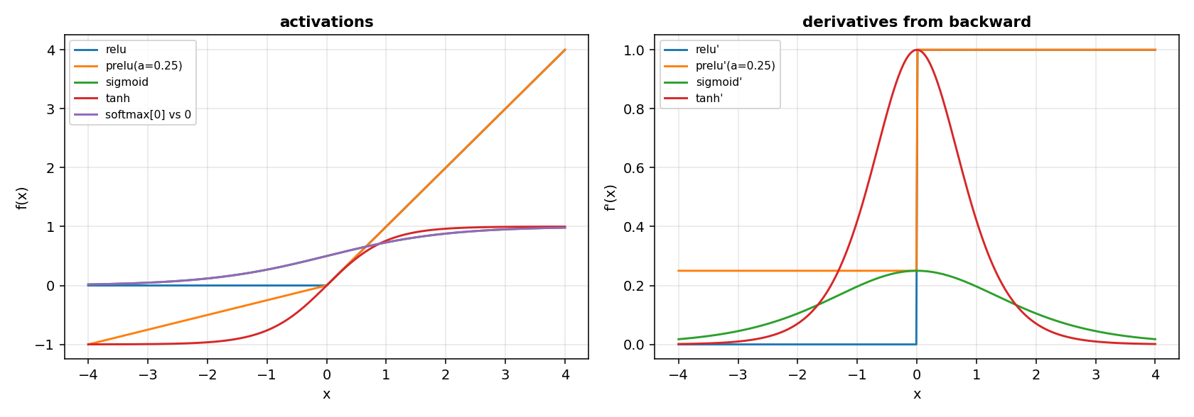
The left panel is the five activations on x in [-4, 4], the right panel the derivative of each one as the code backward returns it.

Details

References

• He, K., Zhang, X., Ren, S., Sun, J. (2015). Delving Deep into Rectifiers: Surpassing Human-Level Performance on ImageNet Classification. arXiv:1502.01852. Page 2, Eqn.(1): the parametric rectifier f(y) = y if y > 0, a*y otherwise. a = 0 is ReLU, a small fixed a is Leaky ReLU. Page 4, Eqn.(10): (1/2) n_l Var[w_l] = 1, a zero-mean Gaussian of standard deviation sqrt(2/n_l), biases zero. Page 5, Eqn.(15): (1/2)(1 + a^2) n_l Var[w_l] = 1, with a = 1 the linear case "the same as [7]", the Xavier initialisation.
• Glorot, X., Bengio, Y. (2010). Understanding the Difficulty of Training Deep Feedforward Neural Networks. AISTATS 2010, PMLR 9:249-256. Page 5, Eqn.(16): the normalised initialisation W ~ U[-√6/√(n_j + n_{j+1}), √6/√(n_j + n_{j+1})]. The PDF is open on the PMLR site. Pages 5 Eqn.(4) to (7) give the forward and backward variance relations, not the initialisation; Eqn.(1), page 3, is the common heuristic U[-1/√n, 1/√n] that the paper compares with, not the normalised initialisation.
• Huber, P. J. (1964). Robust Estimation of a Location Parameter. The Annals of Mathematical Statistics 35(1), 73-101. DOI 10.1214/aoms/1177703732. The PDF is paywalled: the download returns a 1.2 kB HTML paywall page, not a PDF, so only the bibliographic metadata is verified. The formula used by the code is quoted from the open-access secondary source below, page 4.
• Chinot, G. (2019). Robust learning and complexity dependent bounds for regularized problems. arXiv:1902.02238. Page 4: l(u, y) = (1/2)(y - u)**2 if |u - y| <= delta, delta*|y - u| - delta**2/2 otherwise, with the Huber loss L = delta-Lipschitz. The paper is open on arXiv, 38 pages.
• Sigmoid, tanh, softmax, mean squared error, cross-entropy: textbook definitions, no citation.

Choices stated explicitly

• The derivative of ReLU at x = 0 is 0. The paper does not define it, and PyTorch uses 0; this code uses 0.
• The gradient check evaluates the finite differences with eps = 1e-6. The step is large enough that float32 does not lose all digits, small enough that the truncation error of the central difference stays below the tolerance of the tests (1e-7 on a correct pair).
• The gradient check runs inside jax.enable_x64(True) and restores the previous setting at the end. Outside the call the global precision is unchanged.
• The Huber loss and glorot_uniform are optional pieces. The Huber formula is quoted from the open-access Chinot (2019), page 4, because the primary paper (Huber 1964) is paywalled. The Glorot uniform is Glorot and Bengio (2010), Eqn.(16), page 5.
• The layers of the next task (N02: Dense, Conv, RNN) are not delivered. They belong to a separate task, and N01 stops at the pieces that the gradient check tests.

Development diary

The pieces of this delivery are the ones the gradient check can test end to end. The Huber loss and glorot_uniform are optional, and the page states it: the first is outside N01 and quoted from Chinot (2019), page 4, the second is the normalised uniform of Glorot and Bengio (2010), page 5. The layers of N02 (Dense, Conv, RNN) belong to a separate task and are not delivered here.

The first version of the gradient check divided each difference by the analytic gradient rather than by the sum of the absolute values, and a single element with a small analytic gradient made the relative error large even when the backward was right. The division by max(|a| + |b|, 1e-12) keeps the error at the scale of the values compared.

The five activations and the three losses were written before their classes, because the classes need the functions and the tests work on the functions. The classes cache the last x and y; calling backward before forward raises RuntimeError and a test exercises the guard for each class.