Chains: how do I join layers into a network and train it one sample at a time or on a batch?

A layer takes a vector and returns a vector. A network is layers joined end to end: the output of one is the input of the next. This page builds the two containers that do the joining, a chain and a branching, and two classic networks from them, the MLP and the residual MLP. Every container is itself a layer, with forward, backward and params(), so a container goes inside another container, inside a Residual, and inside the streaming interface of the library. The same code trains on a batch of joint states and on one state at a time.

The layers are the ones of the page neural/layers.md, on a synthetic stream of joint states: positions q, velocities qd, torques tau, at a fixed rate, labelled synthetic.

1. A chain of layers

A chain applies its layers in order. The forward pass runs from the first layer to the last, the backward pass from the last to the first, and the gradient of a layer is the gradient the next layer sends back.

import jax
import jax.numpy as jnp
from dense_armor.utility.neural.chain import Sequential
from dense_armor.utility.neural.layers import Dense
from dense_armor.utility.neural.activations import Relu

s = Sequential([Dense(3, 4, jax.random.PRNGKey(0)), Relu(),
                Dense(4, 2, jax.random.PRNGKey(1))])
x = jnp.ones(3)
print(s.forward(x).shape, len(s))

(2,) 3

A chain of three layers takes a vector of length 3 and returns a vector of length 2. params() returns the parameters of every layer in order, zero_grad() sets their gradients to zero, and backward(g) returns the gradient of the input.

2. The same code, on a batch and on one sample

A chain works on a batch and on a single sample with the same forward and backward. A vector of length n_in gives a vector of length n_out; a batch of shape (m, n_in) gives a batch of shape (m, n_out). The single sample is the matching row of the batch.

import numpy as np
import jax
import jax.numpy as jnp
from dense_armor.utility.neural.chain import Sequential
from dense_armor.utility.neural.layers import Dense

s = Sequential([Dense(3, 2, jax.random.PRNGKey(0))])
xb = jnp.array([[1.0, 2.0, 3.0], [4.0, 5.0, 6.0]])
yb = s.forward(xb)
y1 = s.forward(xb[0])
print(np.allclose(np.asarray(y1), np.asarray(yb[0])))

True

The batch and the single sample give the same output. The gradient has the same property: the gradient of a mean loss on a batch is the sum of the gradients of the samples, taken one at a time and divided by the batch size.

import numpy as np
import jax
import jax.numpy as jnp
from dense_armor.utility.neural.chain import Sequential
from dense_armor.utility.neural.layers import Dense

s = Sequential([Dense(3, 2, jax.random.PRNGKey(0))])
xb = jnp.ones((4, 3))
s.zero_grad()
yb = s.forward(xb)
s.backward(jnp.ones_like(yb) / 4.0)
g_batch = [np.array(p.grad) for p in s.params()]

s.zero_grad()
for row in xb:
    y = s.forward(row)
    s.backward(jnp.ones_like(y) / 4.0)
g_online = [np.array(p.grad) for p in s.params()]
print(all(np.allclose(a, b, atol=1e-5) for a, b in zip(g_batch, g_online)))

True

This is why the same training loop works on a batch and on a stream: the gradient of the mean loss is the average of the per-sample gradients, and the two ways of taking it agree to 1e-5.

A small case by hand

A chain of two layers with the weights written down, to see what backward returns. Dense(2, 2) with W1 = [[1, 2], [3, 4]] and zero bias, a Relu, then Dense(2, 1) with W2 = [[5], [6]] and zero bias. The input is two samples, X = [[1, 2], [3, 4]], and the targets are T = [[90], [200]]. The loss is the mean squared error.

The forward pass is H = X W1 = [[7, 10], [15, 22]]; the rectifier leaves it unchanged, since both columns are positive; and Y = H W2 = [[95], [207]]. The gradient of the loss with respect to Y, for L = mean((Y - T)^2), is g = (Y - T) / 2 = [[2.5], [3.5]].

import numpy as np
import jax
import jax.numpy as jnp
from dense_armor.utility.neural.chain import Sequential
from dense_armor.utility.neural.layers import Dense
from dense_armor.utility.neural.activations import Relu

d1 = Dense(2, 2, jax.random.PRNGKey(0))
d1.W.value = jnp.array([[1.0, 2.0], [3.0, 4.0]])
d1.b.value = jnp.array([0.0, 0.0])
d2 = Dense(2, 1, jax.random.PRNGKey(1))
d2.W.value = jnp.array([[5.0], [6.0]])
d2.b.value = jnp.array([0.0])
s = Sequential([d1, Relu(), d2])

X = jnp.array([[1.0, 2.0], [3.0, 4.0]])
T = jnp.array([[90.0], [200.0]])
Y = s.forward(X)
g = (Y - T) / X.shape[0]
s.zero_grad()
dx = s.backward(g)
print(np.asarray(Y).tolist())
print(np.asarray(d1.W.grad).tolist())
print(np.asarray(dx).tolist())

[[95.0], [207.0]]
[[65.0, 78.0], [95.0, 114.0]]
[[42.5, 97.5], [59.5, 136.5]]

The same numbers by hand, step by step: dW2 = relu(H)^T g = [[70], [102]] and db2 = g.sum(axis=0) = [6]; dH = g W2^T * mask = [[12.5, 15], [17.5, 21]], where the mask is 1 because both entries of H are positive; dW1 = X^T dH = [[65, 78], [95, 114]] and db1 = dH.sum(axis=0) = [30, 36]; and dx = dH W1^T = [[42.5, 97.5], [59.5, 136.5]]. The test test_chain_two_layers_gradient_by_hand in test/neural/test_chain.py checks all five arrays against these numbers within 1e-6.

3. Branches that merge

A branching sends the same input to several branches and merges the outputs. With merge="add" the outputs are summed, so every branch must return the same shape. With merge="concat" the outputs are concatenated on the last axis, so the branches can return different widths.

import jax
import jax.numpy as jnp
from dense_armor.utility.neural.chain import Parallel
from dense_armor.utility.neural.layers import Dense

d1 = Dense(3, 4, jax.random.PRNGKey(0))
d2 = Dense(3, 4, jax.random.PRNGKey(1))
p = Parallel([d1, d2], "add")
x = jnp.ones(3)
print(p.forward(x).shape)

(4,)

Two branches of width 4, summed, still give a vector of width 4. With concat the widths add up.

import jax
import jax.numpy as jnp
from dense_armor.utility.neural.chain import Parallel
from dense_armor.utility.neural.layers import Dense

p = Parallel([Dense(3, 4, jax.random.PRNGKey(0)),
              Dense(3, 2, jax.random.PRNGKey(1))], "concat")
print(p.forward(jnp.ones(3)).shape)

(6,)

The backward pass of "add" passes the same g to every branch and sums the gradients of the input; the backward pass of "concat" splits g by the width of each branch. A branch of a different width with "add" raises ValueError, because the sum is not defined.

A chain and a branching are layers, so they combine: a Parallel inside a Sequential, a Sequential inside a Parallel, a Parallel inside a Residual.

4. The MLP

An MLP is a chain of dense layers with an activation between them. The function builds it from a list of widths, from the input to the output; the last dense layer has no activation after it, because the activation is the job of the loss.

import jax
from dense_armor.utility.neural.models import mlp

m = mlp([2, 8, 1], jax.random.PRNGKey(0))
print([p.value.shape for p in m.params()])

[(2, 8), (8,), (8, 1), (1,)]

The chain has two dense layers (the (2, 8) and the (8, 1) with their biases) and one activation between them, which has no parameters. The activation is "relu" by default; "tanh" and "sigmoid" are also accepted. A list of one width, or an activation that is not one of the three names, raises ValueError.

The initialisation follows the activation. He et al. 2015 (Eqn.(15), page 5) derive the variance for the rectifier and name the linear case as Xavier. The dense layers use "he" with relu and "xavier" with tanh and sigmoid. This is our choice, stated in the docstring of mlp.

5. The residual MLP

A residual MLP is a chain of blocks. Each block is a chain of a Residual around two dense layers with a rectifier between them, followed by a rectifier: the block of Figure 2, page 2 of He et al. 2016 with the addition y = F(x) + x of Eqn.(1), page 3.

import jax
from dense_armor.utility.neural.models import resnet_mlp

r = resnet_mlp(8, 2, 3, 2, jax.random.PRNGKey(0))
print(len(r.params()))

12

A network with two blocks has 12 parameters: a Dense(3, 8) and its bias (2), two blocks with two dense layers each (4 parameters per block, 8), and a final Dense(8, 2) and its bias (2). The blocks have no normalisation: the block of the figure is written for convolutions, and this is the dense form. This is our choice, stated in the docstring.

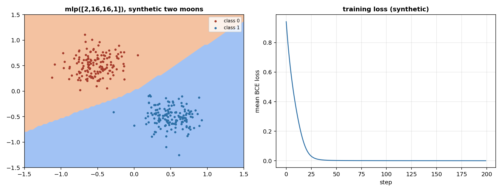
The left panel is the decision boundary of mlp([2, 16, 16, 1]) after 200 steps of Adam on a synthetic two-moons set; the right panel is the mean binary cross-entropy against the step, from the same run, with final loss 0.0003. The set is made by the script, labelled synthetic in the title of both panels.

Details

References

• He, K., Zhang, X., Ren, S., Sun, J. (2016). Deep Residual Learning for Image Recognition. arXiv:1512.03385. Page 2, Figure 2: the residual building block. Page 3, Eqn.(1): y = F(x, {W_i}) + x, with the note that the dimensions of x and F must be equal.
• He, K., Zhang, X., Ren, S., Sun, J. (2015). Delving Deep into Rectifiers. arXiv:1502.01852. Page 5, Eqn.(15): (1/2)(1 + a**2) n_l Var[w_l] = 1, with a = 0 the rectifier case and a = 1 the linear case named Xavier.
• The chain rule applied in reverse order, the sum of the gradients of the samples of a batch, the XOR problem and the two-moons set are textbook definitions and carry no citation.

Choices stated explicitly

• Sequential tests once, when it is built, whether a layer's forward accepts training, and calls it either as forward(x, training=training) or as forward(x). The test is made with inspect.signature, and a layer whose forward has a **kwargs also receives training.
• Parallel is the only branching form. A general graph with shared nodes, where the same layer is reachable from more than one path, is not built: a shared layer would accumulate its gradient twice in a naive sum, and a correct shared-node backward needs an explicit graph traversal that this page does not have.
• mlp uses "he" with relu and "xavier" with tanh and sigmoid. The reason is in section 4: He et al. 2015 derive the variance for the rectifier and name the linear case as Xavier.
• The block of resnet_mlp has no normalisation. The block of Figure 2 of He et al. 2016 is written for convolutions; this is the dense form, and adding a normalisation layer would be our choice, not the paper's.
• The two-moons set in benchmarks/neural/chains_figure.py is made by a function of the script, with a fixed seed, labelled synthetic.

Development diary

The delivery leaves out the convolutional network, the recurrent network and the transformer block, which need the layers of N02b and the attention of N07: task N03b. A general graph with shared nodes is also left out, as stated in the Choices.