Recurrent layers and attention: how do I keep a memory of the past samples?
A feed-forward network sees each input on its own. A recurrent network sees a sequence and keeps a hidden state from one step to the next: the output at step t depends on the input at step t and on the state the network carried from steps 0 to t - 1. This is the right tool for a stream of joint states sampled at a fixed rate, where the velocity of the joint at step t is read from the last few samples. Attention is a second way to mix the samples of a sequence, without a recurrent state: every position looks at every other position, weighted by a learned similarity. A transformer block stacks attention and a feed-forward network with residual connections.
The examples in this page use a synthetic sequence of 5 steps of width 4 (one sample per step, labelled synthetic), the kind of window a robot arm's sensors give after a small crop. A recurrent layer or a block takes the whole window and returns a vector per step, or a single vector with the last step or the mean.
1. One GRU step, by hand
The GRU of Cho et al. 2014 has a reset gate r, an update gate z and a candidate hidden state. The equations are Eqs.(5) to (8), page 3:
r = sigmoid(W_r x + U_r h_prev), z = sigmoid(W_z x + U_z h_prev), h_tilde = tanh(W x + U (r * h_prev)), h = z * h_prev + (1 - z) * h_tilde.
A 1-input, 1-hidden case with weights written down shows the numbers. W_r = 1, U_r = 0; W_z = 1, U_z = 0; W = 2, U = 1; all biases zero. x_t = 1.0, h_prev = 0.5.
import jax
import jax.numpy as jnp
from dense_armor.utility.neural.recurrent import GRU

g = GRU(1, 1, jax.random.PRNGKey(0))
g.W_r.value = jnp.array([[1.0]]); g.U_r.value = jnp.array([[0.0]]); g.b_r.value = jnp.array([0.0])
g.W_z.value = jnp.array([[1.0]]); g.U_z.value = jnp.array([[0.0]]); g.b_z.value = jnp.array([0.0])
g.W.value = jnp.array([[2.0]]); g.U.value = jnp.array([[1.0]]); g.b.value = jnp.array([0.0])
y, _ = g.step(jnp.array([1.0]), jnp.array([0.5]))
print(round(float(y[0]), 4))
The hand computation: r = sigmoid(1) = 0.7311, z = sigmoid(1) = 0.7311, h_tilde = tanh(2 + 1 * 0.7311 * 0.5) = tanh(2.3655) = 0.9821, h = 0.7311 * 0.5 + 0.2689 * 0.9821 = 0.6298. The update gate keeps three quarters of the previous state and mixes in a quarter of the candidate.
2. One LSTM step, by hand
The vanilla LSTM of Greff et al. 2017 (pages 1 and 2) has an input gate i, a forget gate f, an output gate o, a cell c and an output y. With peepholes, i and f see the previous cell c_prev, and o sees the current cell c.
The forward pass of page 2: z = tanh(W_z x + R_z y_prev + b_z), i = sigmoid(W_i x + R_i y_prev + p_i * c_prev + b_i), f = sigmoid(W_f x + R_f y_prev + p_f * c_prev + b_f), c = z * i + c_prev * f, o = sigmoid(W_o x + R_o y_prev + p_o * c + b_o), y = tanh(c) * o.
import jax
import jax.numpy as jnp
from dense_armor.utility.neural.recurrent import LSTM

ls = LSTM(1, 1, jax.random.PRNGKey(0))
for n in ("W_z","W_i","W_f","W_o","R_z","R_i","R_f","R_o","b_z","b_i","b_f","b_o","p_i","p_f","p_o"):
    setattr(getattr(ls, n), "value", jnp.zeros_like(getattr(ls, n).value))
ls.W_z.value = jnp.array([[1.0]]); ls.W_i.value = jnp.array([[1.0]])
ls.W_f.value = jnp.array([[1.0]]); ls.W_o.value = jnp.array([[1.0]])
out, _ = ls.step(jnp.array([0.5]), (jnp.array([0.1]), jnp.array([0.2])))
print(round(float(out[0]), 4))
The hand computation with x = 0.5, y_prev = 0.1, c_prev = 0.2, all biases and peepholes zero: z = tanh(0.5) = 0.4621, i = sigmoid(0.5) = 0.6225, f = sigmoid(0.5) = 0.6225, c = 0.4621 * 0.6225 + 0.2 * 0.6225 = 0.4122, o = sigmoid(0.5) = 0.6225, y = tanh(0.4122) * 0.6225 = 0.2429. The peephole vectors are zero by construction, so the output only depends on the four input weights.
3. The same code on a sequence and on one step
forward runs the whole sequence from a zero state, and step runs one sample from the state of the previous step. The two give the same numbers.
import jax
import jax.numpy as jnp
import numpy as np
from dense_armor.utility.neural.recurrent import GRU

g = GRU(2, 3, jax.random.PRNGKey(0))
seq = jax.random.normal(jax.random.PRNGKey(1), (5, 2))
yf = g.forward(seq)
h = g.init_state()
ys = []
for t in range(5):
    yt, h = g.step(seq[t], h)
    ys.append(yt)
print(bool(np.allclose(np.asarray(jnp.stack(ys)), np.asarray(yf), atol=1e-6)))
forward is what a training loop uses, step is what a control loop uses: the same weights, the same code, the same output. init_state returns the zero state, of shape (n_hidden,) for a single sample and (batch, n_hidden) for a batch. The LSTM has the same interface, with a state that is the pair (y, c).
4. Multi-head self-attention, the shapes
A multi-head self-attention of Vaswani et al. 2017 (page 5) projects the input into queries, keys and values, splits them into n_heads heads of size d_model / n_heads, runs the scaled dot-product attention on each head, concatenates the heads and projects the result. The four projection weights W_Q, W_K, W_V, W_O are learned.
import jax
import jax.numpy as jnp
from dense_armor.utility.neural.attention import MultiHeadSelfAttention

m = MultiHeadSelfAttention(8, 2, jax.random.PRNGKey(0))
print(m.forward(jnp.ones((4, 8))).shape)
print(len(m.params()))
A sequence of shape (4, 8) (4 steps, d_model = 8) gives the same shape back, because self-attention preserves the input dimension. The four parameters are the four projection matrices. A d_model that is not divisible by n_heads raises ValueError.
5. One attention head, by hand
The scaled dot-product attention of Eq.(1), page 4 of Vaswani et al. 2017 is Attention(Q, K, V) = softmax(Q K^T / sqrt(d_k)) V. With one query [1, 0], two keys [1, 0] and [0, 1] (so d_k = 2), and values 10 and 20, the score of the first key is 1/sqrt(2) = 0.7071 and of the second key is 0. The softmax gives weights 0.6698 and 0.3302, and the output is 0.6698 * 10 + 0.3302 * 20 = 13.3024.
import jax.numpy as jnp
import numpy as np
from dense_armor.utility.neural.attention import scaled_dot_product_attention

q = jnp.array([[1.0, 0.0]])
k = jnp.array([[1.0, 0.0], [0.0, 1.0]])
v = jnp.array([[10.0], [20.0]])
y = scaled_dot_product_attention(q, k, v)
print(round(float(y[0, 0]), 4))
The query [1, 0] is closer to the first key [1, 0] than to the second [0, 1], so the first value 10 gets a larger weight than the second 20. The output is between the two values, closer to 10. The scaling 1/sqrt(d_k) keeps the scores small even when the dot product grows, so the softmax stays in a region where its gradient is not negligible.
6. A causal cache, for a stream
With causal = True, the position t attends only to the positions up to t. The method step takes one sample, appends its keys and values to a cache of shape (T, d_model) and returns the output and the new cache. The output of step called T times equals the output of forward on the whole sequence.
import jax
import jax.numpy as jnp
import numpy as np
from dense_armor.utility.neural.attention import MultiHeadSelfAttention

m = MultiHeadSelfAttention(8, 2, jax.random.PRNGKey(0), causal=True)
seq = jax.random.normal(jax.random.PRNGKey(1), (5, 8))
yf = m.forward(seq)
cache = m.init_cache()
ys = []
for t in range(5):
    yt, cache = m.step(seq[t], cache)
    ys.append(yt)
print(bool(np.allclose(np.asarray(jnp.stack(ys)), np.asarray(yf), atol=1e-5)))
The cache grows by one key-value pair per step, and the attention weights of step t are computed only against the keys of steps 0 to t. init_cache returns two arrays of shape (0, d_model). The causal mask of the forward is a lower-triangular boolean matrix, and the same mask is applied inside scaled_dot_product_attention before the softmax (page 5 of the paper).
7. A transformer encoder, from the sequence to a label
A transformer encoder of Vaswani et al. 2017 stacks a dense projection, a positional encoding, depth transformer blocks and a mean over the time axis, followed by a dense head. The transformer_encoder builder returns a Sequential.
import jax
import jax.numpy as jnp
from dense_armor.utility.neural.models import transformer_encoder

m = transformer_encoder(4, 8, 2, 16, 1, 3, jax.random.PRNGKey(0), 16)
print(m.forward(jnp.ones((5, 4))).shape)
A sequence of shape (5, 4) (5 steps, 4 features) gives a single vector of shape (3,). The MeanOverTime collapses the time axis, and the final Dense(8, 3) gives the three outputs.
8. A recurrent network, from the sequence to a label
A recurrent network of n_layers LSTM, GRU or RNN layers, followed by LastStep and a dense head, is the second classic form. The recurrent_net builder returns a Sequential.
import jax
import jax.numpy as jnp
from dense_armor.utility.neural.models import recurrent_net

m = recurrent_net(3, 4, 2, jax.random.PRNGKey(0))
print(m.forward(jnp.ones((5, 3))).shape)
print(len(m.params()))
A sequence of shape (5, 3) gives a vector of shape (2,). The 17 parameters are the 15 of the LSTM (four weight matrices W, four recurrent matrices R, four biases b, three peepholes p) plus two of the final Dense(4, 2). With cell="gru" the count is 11, with cell="rnn" it is 5: the three cells have 9, 9, 3 parameters respectively, plus the two of the head.
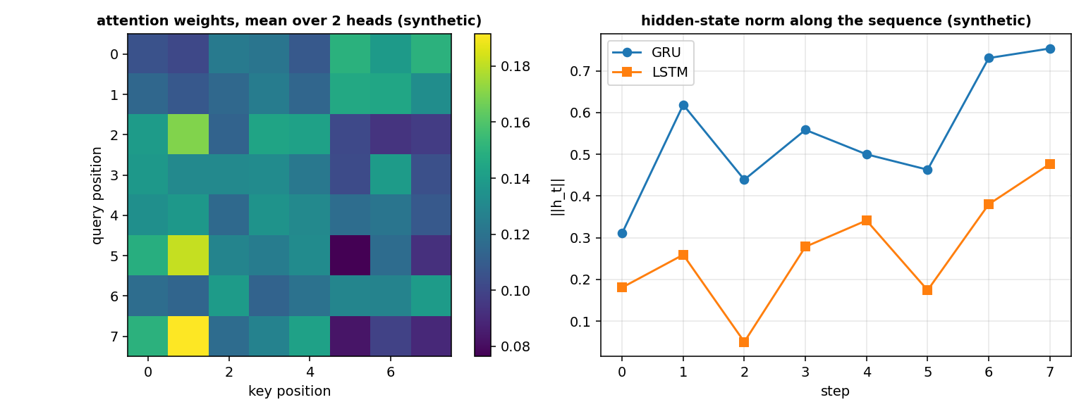
The left panel is the attention weights of a MultiHeadSelfAttention with d_model = 4 and 2 heads on a synthetic sequence of 8 steps, averaged over the heads. The right panel is the norm of the hidden state of a GRU and of an LSTM along the same sequence; the GRU ends at 0.7536 and the LSTM at 0.4770, with a different shape because the two cells carry different amounts of information.
Details
References
- Cho, K., van Merriënboer, B., Gulcehre, C., Bahdanau, D., Bougares, F., Schwenk, H., Bengio, Y. (2014). Learning Phrase Representations using RNN Encoder-Decoder for Statistical Machine Translation. arXiv:1406.1078. Page 3, Eqs.(5) to (8), the reset gate, the update gate, the candidate and the hidden state.
- Greff, K., Srivastava, R. K., Koutník, J., Steunebrink, B. R., Schmidhuber, J. (2017). LSTM: A Search Space Odyssey. arXiv:1503.04069. Page 1, the vanilla LSTM block and the peephole connections; page 2, the forward formulas and the deltas of the backpropagation through time.
- Vaswani, A., Shazeer, N., Parmar, N., Uszkoreit, J., Jones, L., Gomez, A. N., Kaiser, Ł., Polosukhin, I. (2017). Attention Is All You Need. arXiv:1706.03762. Page 3,
LayerNorm(x + Sublayer(x)); page 4, Eq.(1); page 5, the multi-head attention, the masking and Eq.(2); page 6, the sinusoidal positional encoding. - He, K., Zhang, X., Ren, S., Sun, J. (2016). Deep Residual Learning for Image Recognition. arXiv:1512.03385. Page 2, Figure 2; page 3, Eqn.(1), for the residual connection of a transformer block.
The Elman layer, the last-step and mean-over-time selections and the synthetic tasks are textbook definitions and carry no citation.
Choices stated explicitly
- A
GRUadds a bias to each of the three pre-activations. The paper (page 3) writes no bias; the bias starts at zeros. This is our choice. - The three recurrent layers initialise the input and the recurrent weights with
xavier_normal, and the biases at zeros. The sources are silent on the initialisation; the reason is that the variance of the input and of the hidden state should be the same order of magnitude. This is our choice. - The
LSTMfollows the vanilla block of Greff et al. 2017 (pages 1 and 2) with the peepholes on by default.peepholes = Falseremoves the three peephole vectors, as the paper mentions on page 1. - The
TransformerBlockapplies the dropout on the output of each sub-layer before the addition, as page 8 of the paper does. The default of the block isdropout = 0.0(no dropout), because this page runs on synthetic data and the dropout is only useful at scale. - A
MultiHeadSelfAttentionwithcausal = Truebuilds a lower-triangular mask and passes it toscaled_dot_product_attention, which sets the masked positions to-infbefore the softmax (page 5). Thestepmethod uses the cache of the past and no mask, since the future is not there yet. - The
recurrent_netand thetransformer_encodersplit the key with onejax.random.splitper layer with weights. TheAddPositionshas no weights and does not consume a key.
Development diary
The delivery leaves out the cross-attention and the gate between two signals (task N07), the learned positional encodings, the bidirectional layers and the transposed convolutions (task N03b). An AsTransformer around a recurrent_net or a transformer_encoder is not required by this task and is not provided; the two builders return a Sequential and are not wrapped in a library role.