Training: how do I train a network on a dataset I already have, and stop it before it memorises?

A network of Dense, Residual and Sequential is a function with a set of weights. Training the network means: take a dataset of inputs and labels, feed a batch of inputs, compute the loss, backpropagate, and update the weights by a small step. Repeat for a number of epochs. As the training progresses, the learning rate should go down (slowly at first, then faster, then up again); the weights should shrink slightly to prevent memorisation; and the training should stop before the network starts to fit the noise of the training set instead of the pattern.

This page builds the four pieces: the schedules of the learning rate, the mini-batch generator that turns a dataset into a sequence of index arrays, the trainer that runs the loop with weight decay and early stopping, and a figure that shows the train and validation loss along the epochs. The page works on a synthetic dataset: 40 samples of two features, the label being x0 + 0.5 x1, labelled synthetic in the figure. Real robot data has the same structure, one row per sample.

1. Three learning-rate schedules

A schedule is a function of the epoch (which can be fractional, because the trainer reads it at each batch) that returns a learning rate. The ConstantLR keeps the same rate. The StepLR drops by a factor every step epochs. The CosineWarmRestarts drops along a cosine and restarts every t0 epochs.

from dense_armor.utility.neural.schedules import (
    ConstantLR, StepLR, CosineWarmRestarts,
)
print(ConstantLR(0.1)(5.0))
print(StepLR(0.1, 10, 0.5)(25.0))
c = CosineWarmRestarts(0.05, 0.0, 5)
print(round(c(0.0), 4), round(c(2.5), 4), round(c(5.0), 4))

0.1
0.025
0.05 0.025 0.05

ConstantLR(0.1) returns 0.1 at any epoch. StepLR(0.1, 10, 0.5) at epoch 25 returns 0.1 * 0.5 ** floor(25/10) = 0.1 * 0.5**2 = 0.025. CosineWarmRestarts(0.05, 0.0, 5) starts at 0.05, drops to 0.025 at the midpoint of the first run (epoch 2.5), and goes back to 0.05 at epoch 5 (the restart). Within the run i, lr = lr_min + (1/2)(lr_max - lr_min)(1 + cos(pi * t_cur / t_i)) (Eqn.(5), page 4 of Loshchilov and Hutter 2017), where t_cur is the number of epochs since the last restart and t_i = t0 * t_mult ** i.

2. Mini-batches from a dataset

A mini-batch generator takes the length n of the dataset and the size batch_size and yields arrays of indices. With a jax.random key the order is a permutation, so every epoch sees a different order; without a key the order is 0, 1, ..., n-1.

from dense_armor.utility.neural.batching import minibatches
print([b.tolist() for b in minibatches(10, 3)])
print([len(b) for b in minibatches(10, 3, drop_last=True)])

[[0, 1, 2], [3, 4, 5], [6, 7, 8], [9]]
[3, 3, 3]

Without drop_last, the last batch is [9], shorter than the others. With drop_last=True, the last batch is not yielded, and the three full batches remain. batch_size larger than n gives a single batch with all the indices.

3. The trainer

A Trainer wraps a model (any object with forward, backward and params()) and a loss (any object with forward(pred, target) and backward()), and runs fit(X, y, epochs, batch_size, key) over the dataset. For each epoch, the trainer splits the data into mini-batches, computes the loss of each batch, backpropagates, and updates every Param. The history of the training is in history_: a dict with the train_loss and lr of each epoch.

import jax
import numpy as np
from dense_armor.utility.neural.trainer import Trainer
from dense_armor.utility.neural.models import mlp
from dense_armor.utility.neural.losses import MSE
from dense_armor.utility.optim import SGD

rng = np.random.default_rng(0)
X = rng.normal(0.0, 1.0, (40, 2)).astype(np.float32)
y = (X[:, 0:1] + 0.5 * X[:, 1:2]).astype(np.float32)
m = mlp([2, 8, 1], jax.random.PRNGKey(0))
t = Trainer(m, MSE(), SGD(0.05))
t.fit(X, y, epochs=5, batch_size=10, key=jax.random.PRNGKey(1))
print(len(t.history_["train_loss"]))
print(round(t.history_["train_loss"][0], 4), round(t.history_["train_loss"][-1], 4))
print(round(t.history_["lr"][0], 4))

5
7.5319 0.1299
0.05

The history has 5 entries, one per epoch. The loss drops from 7.5319 in the first epoch to 0.1299 in the last. The learning rate of the first batch of the first epoch is 0.05, the default of SGD. The Trainer copies the optimizer for each Param, because the object form of SGD and Adam holds the state of one array, and every Param needs its own copy.

4. Weight decay: L2 and decoupled

Weight decay shrinks the weights slightly at each step, to prevent them from growing too large and memorising the training set. There are two forms. L2 adds weight_decay * value to the gradient, before the update: the shrinkage is part of the gradient, and the optimizer treats it as one of its terms (Algorithm 1, line 6, page 3 of Loshchilov and Hutter 2019). Decoupled subtracts eta_t * weight_decay * value from the weights directly, after the update (Algorithm 1, line 9, and Algorithm 2, line 12, of the same paper). For standard SGD with learning rate alpha, the two forms are equivalent when the L2 coefficient is lambda / alpha for a decoupled decay lambda (Proposition 1, page 2).

import jax
import numpy as np
from dense_armor.utility.neural.trainer import Trainer
from dense_armor.utility.neural.models import mlp
from dense_armor.utility.neural.losses import MSE
from dense_armor.utility.optim import SGD

rng = np.random.default_rng(0)
X = rng.normal(0.0, 1.0, (20, 2)).astype(np.float32)
y = rng.normal(0.0, 1.0, (20, 1)).astype(np.float32)

ml = mlp([2, 4, 1], jax.random.PRNGKey(0))
tl = Trainer(ml, MSE(), SGD(0.1), weight_decay=1.0, decay="l2")
tl.fit(X, y, epochs=3, batch_size=20, key=jax.random.PRNGKey(0), shuffle=False)

md = mlp([2, 4, 1], jax.random.PRNGKey(0))
td = Trainer(md, MSE(), SGD(0.1), weight_decay=0.1, decay="decoupled")
td.fit(X, y, epochs=3, batch_size=20, key=jax.random.PRNGKey(0), shuffle=False)

d = max(float(np.max(np.abs(np.asarray(a.value) - np.asarray(b.value))))
        for a, b in zip(ml.params(), md.params()))
print(f"{d:.2e}")

5.96e-08

The two trainers leave the weights equal within 5.96e-08, because with alpha = 0.1 and lambda = 0.1 the L2 coefficient lambda / alpha = 1.0 is the one the first trainer uses. The equivalence holds for standard SGD; with Adam it does not, and the two forms leave different weights. The weight decay applies only to the Param whose value has two or more dimensions, so the biases, the gains and the offsets are not shrunk.

5. Early stopping

With a validation set and a patience, the trainer stops at the end of the epoch after which the validation loss has not improved by min_delta for patience consecutive epochs. The weights are restored to those of the best epoch, so the final model is the one that generalised best, not the last one.

import jax
import numpy as np
from dense_armor.utility.neural.trainer import Trainer
from dense_armor.utility.neural.models import mlp
from dense_armor.utility.neural.losses import MSE
from dense_armor.utility.optim import Adam

rng = np.random.default_rng(0)
X = rng.normal(0.0, 1.0, (40, 2)).astype(np.float32)
y = rng.normal(0.0, 1.0, (40, 1)).astype(np.float32)
Xv = rng.normal(0.0, 1.0, (20, 2)).astype(np.float32)
yv = rng.normal(0.0, 1.0, (20, 1)).astype(np.float32)

m = mlp([2, 16, 16, 1], jax.random.PRNGKey(0))
t = Trainer(m, MSE(), Adam(0.01))
t.fit(X, y, epochs=100, batch_size=10, key=jax.random.PRNGKey(0),
      X_val=Xv, y_val=yv, patience=5)
print(t.stopped_epoch_, t.best_epoch_)
print(abs(t.evaluate(Xv, yv) - t.history_["val_loss"][t.best_epoch_]) < 1e-5)

8 3
True

The training stops at epoch 8, the best epoch is 3, and the evaluate on the validation set after the fit equals the val_loss recorded at the best epoch (within 1e-5). Without patience, the same run does all 100 epochs and the weights stay as the last epoch left them. patience without a validation set, patience < 1, epochs < 1 and X and y of different lengths raise ValueError.

6. Evaluate and predict

The trainer also provides evaluate(X, y), which computes the loss of the whole set with training=False, and predict(X), which returns the output of the model with training=False.

import jax
import jax.numpy as jnp
from dense_armor.utility.neural.trainer import Trainer
from dense_armor.utility.neural.models import mlp
from dense_armor.utility.neural.losses import MSE
from dense_armor.utility.optim import SGD

X = jnp.ones((4, 2))
y = jnp.zeros((4, 1))
m = mlp([2, 4, 1], jax.random.PRNGKey(0))
t = Trainer(m, MSE(), SGD(0.01))
t.fit(X, y, epochs=2, batch_size=2, key=jax.random.PRNGKey(0))
print(t.predict(X).shape)
print(round(t.evaluate(X, y), 4) >= 0.0)

(4, 1)
True

predict returns the same shape as the model's output, evaluate returns a float that is non-negative (MSE). The two calls use training=False, so Dropout and BatchNorm are in evaluation mode.

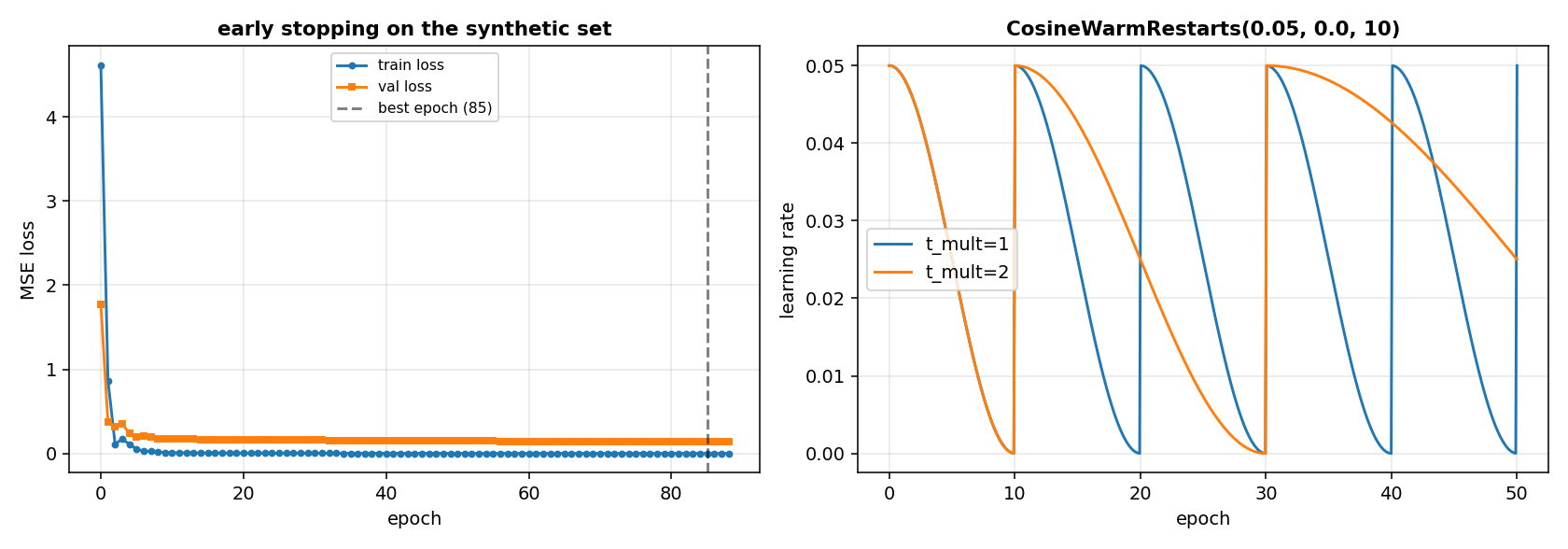
The left panel is the train and validation loss of mlp([2, 16, 16, 1]) trained with Adam on the synthetic set, with early stopping at the best epoch (a vertical dashed line). The right panel is the learning rate of CosineWarmRestarts(0.05, 0.0, 10) with t_mult=1 and t_mult=2: the first restarts every 10 epochs, the second doubles the period at each restart.

Details

References

• Loshchilov, I., Hutter, F. (2017). SGDR: Stochastic Gradient Descent with Warm Restarts. arXiv:1608.03983. Page 4, Eqn.(5), the cosine annealing within a run; page 2, Figure 1, the schedules with t_mult = 1 and t_mult = 2.
• Loshchilov, I., Hutter, F. (2019). Decoupled Weight Decay Regularization. arXiv:1711.05101. Page 2, Eqn.(1), the weight decay and Proposition 1, the equivalence with L2 regularisation for standard SGD (lambda' = lambda / alpha); page 3, Algorithm 1, line 6 for the gradient with the L2 term and line 9 for the decoupled decay, Algorithm 2, line 12 for Adam.

The mini-batch loop, the shuffling by a permutation, the step schedule, the early-stopping rule and the two-moons set are textbook definitions and carry no citation.

Choices stated explicitly

• One copy.deepcopy of the optimizer for each Param. The object form of SGD and Adam holds the state of one array (the first moment, the second moment, the step counter of Adam), so a single instance cannot serve two Param of different shape. Each copy sees only its own Param.
• The default schedule is ConstantLR(optimizer.lr), with the learning rate of the optimizer prototype. A user who passes a different schedule overrides the default.
• The weight decay applies only to the Param whose value has two or more dimensions, so the biases, the gains and the offsets are not shrunk. This is the convention of the reference frameworks and the one the paper mentions for its own experiments.
• The early-stopping rule is the textbook one: the training stops when the validation loss has not improved by min_delta for patience consecutive epochs, and the weights of the best epoch are restored. The paper is silent on the exact rule; this is our choice.
• The Trainer uses minibatches with a new jax.random.split for the shuffle at each epoch. With shuffle=False, no key is passed and the order is 0, 1, ..., n-1.
• The lr of the history is the learning rate of the first batch of the epoch. The learning rate is set on every optimizer copy at every batch, and the schedule is evaluated at the fractional epoch epoch + b / n_batches.

Development diary

The delivery leaves out the online training with learn_one, the checkpoints and the latency budget (task N05), the gradient clipping, the mixed precision and the early-stopping rule with a moving average of the validation loss. The Trainer is a single class, not a hierarchy: an EarlyStopping callback would be a separate abstraction, out of this task's scope.