Continuous training: how do I keep a network learning from a stream, without blocking the loop and without losing it when the program stops?
A robot produces a sample at a fixed rate: the joint positions, the velocities and the torques at step t, as a dict of a few numbers. The model must learn from that sample before the next one arrives, and must predict between two samples without waiting for the training. The Trainer of the page neural/training.md runs epochs over a whole dataset, which is what a training job does, not what a control loop does. The online mode of this page is the same step as the Trainer with a batch of one sample, called by learn_one(x, y) on a single sample.
This page builds the four pieces: the online estimators (OnlineNetRegressor, OnlineNetClassifier), the Hedge Backpropagation network that chooses its depth while it runs, the background learner that moves the training to a worker thread, and a checkpoint saved and restored between two runs of the program. The page works on a synthetic stream of joint states (q, qd, tau at 100 Hz, labelled synthetic).
1. The online step, by hand
OnlineNetRegressor.learn_one(x, y) performs the same step as one batch of Trainer.fit with batch_size=1: zero the gradient, forward, loss, backward, the learning rate from a schedule, the weight decay, the update. A Dense(1, 1) with W = 2.0 and b = 0.0, the sample x = 1.0, y = 0.0, the mean squared error and SGD(0.1) give W = 1.6 and b = -0.4 after one step.
import jax
import jax.numpy as jnp
from dense_armor.utility.neural.online import OnlineNetRegressor
from dense_armor.utility.neural.layers import Dense
from dense_armor.utility.neural.losses import MSE
from dense_armor.utility.optim import SGD

d = Dense(1, 1, jax.random.PRNGKey(0))
d.W.value = jnp.array([[2.0]])
d.b.value = jnp.array([0.0])
r = OnlineNetRegressor(d, MSE(), SGD(0.1), feature_keys=["x"])
r.learn_one({"x": 1.0}, 0.0)
print(round(float(r.model_.params()[0].value[0, 0]), 2))
print(round(float(r.model_.params()[1].value[0]), 2))
The forward pass gives 2.0. The gradient of the MSE with respect to the prediction is 2 * (2.0 - 0.0) = 4.0. With a dense layer dW = x * g = 4.0, so the new weight is 2.0 - 0.1 * 4.0 = 1.6; the new bias is 0.0 - 0.1 * 4.0 = -0.4. The same numbers a Trainer with a batch of one sample would give.
2. The online step equals the batch of one sample
Twenty samples fed one by one to OnlineNetRegressor leave the weights equal, within 1e-6, to one Trainer.fit with batch_size=1 and shuffle=False on the same model and the same data. This is the contract of N04: one code path serves the batch mode and the online mode.
import jax
import numpy as np
from dense_armor.utility.neural.online import OnlineNetRegressor
from dense_armor.utility.neural.trainer import Trainer
from dense_armor.utility.neural.models import mlp
from dense_armor.utility.neural.losses import MSE
from dense_armor.utility.optim import SGD

rng = np.random.default_rng(0)
X = rng.normal(0.0, 1.0, (10, 2)).astype(np.float32)
y = (X[:, 0] + 0.5 * X[:, 1]).astype(np.float32)

m1 = mlp([2, 4, 1], jax.random.PRNGKey(42))
t = Trainer(m1, MSE(), SGD(0.1))
t.fit(X, y.reshape(-1, 1), epochs=1, batch_size=1,
      key=jax.random.PRNGKey(0), shuffle=False)
w_t = [np.asarray(p.value) for p in m1.params()]

m2 = mlp([2, 4, 1], jax.random.PRNGKey(42))
o = OnlineNetRegressor(m2, MSE(), SGD(0.1), feature_keys=["a", "b"])
for i in range(10):
    o.learn_one({"a": float(X[i, 0]), "b": float(X[i, 1])}, float(y[i]))
w_o = [np.asarray(p.value) for p in o.model_.params()]
d = max(float(np.max(np.abs(a - b))) for a, b in zip(w_t, w_o))
print(f"{d:.2e}")
The two paths give the same weights to machine precision. The classifier (OnlineNetClassifier) uses BCEWithLogits for two classes and SoftmaxCrossEntropy for more, and predict_proba_one returns the class probabilities. A sample with a missing feature, None, NaN, a non-numeric value or a non-finite target is counted in n_missing_ and does not change the weights.
3. Hedge Backpropagation, the depth chosen while it runs
A Hedge network of Sahoo, Pham, Lu and Hoi (2018) has L + 1 classifiers on the representations h(0) = x, h(l) = relu(W(l) h(l-1)), each with a softmax output f(l) = softmax(h(l) Theta(l)). The prediction is F(x) = sum_l alpha(l) f(l)(x), a weighted sum of the depths (Eq.(1), page 3). The alpha(l) start uniform, and after every sample they are discounted by beta ** L(l), where L(l) = 1 - p(l)[y] is the loss of the classifier at depth l, then smoothed to s / L and normalised to sum to 1 (page 4).
import jax
import numpy as np
from dense_armor.utility.neural.hedge import HedgeNetClassifier

c = HedgeNetClassifier([2, 4, 4, 4], jax.random.PRNGKey(0), classes=[0, 1])
print(c.L_)
print(np.round(np.asarray(c.alphas_), 3).tolist())
Three hidden layers (L = 3) give four classifiers (depth 0, 1, 2, 3), each with alpha = 1/4 = 0.25. The alphas_ sum to 1 from the first sample.
On a stream where the pattern is linear, the shallow classifiers generalise well after 300 samples: their alphas_ are larger than the deepest, so the network chooses the depth it needs.
import jax
import numpy as np
from dense_armor.utility.neural.hedge import HedgeNetClassifier

rng = np.random.default_rng(0)
X = rng.normal(0.0, 1.0, (300, 2)).astype(np.float32)
y = (X[:, 0] + X[:, 1] > 0.0).astype(int)

c = HedgeNetClassifier([2, 8, 8, 8], jax.random.PRNGKey(0),
                        classes=[0, 1], beta=0.99, lr=0.05,
                        feature_keys=["a", "b"])
for i in range(300):
    c.learn_one({"a": float(X[i, 0]), "b": float(X[i, 1])}, int(y[i]))
print([round(float(v), 3) for v in c.alphas_])
The two shallow classifiers (0 and 1) together hold 0.501, more than the deepest (0.252). The network of L = 3 hidden layers has chosen the depth that fits the linear pattern. The learn_one performs the update of Eq.(2) for Theta(l) and Eq.(3) for W(l) with the sum over j >= l (page 4), and the alphas_ after the smoothing and the normalisation.
4. The background learner, so the main program is never blocked
BackgroundLearner wraps any estimator with learn_one and predict_one and moves the training to a daemon worker thread. The main program puts the sample in a queue.Queue and returns at once; when the queue is full, the oldest sample is dropped and counted in n_dropped_, so the main program never waits and the newest data are kept.
from dense_armor.utility.neural.background import BackgroundLearner
from dense_armor.utility.neural.online import OnlineNetRegressor
from dense_armor.utility.neural.models import mlp
from dense_armor.utility.neural.losses import MSE
from dense_armor.utility.optim import SGD
import jax

m = mlp([2, 4, 1], jax.random.PRNGKey(0))
inner = OnlineNetRegressor(m, MSE(), SGD(0.01), feature_keys=["a", "b"])
b = BackgroundLearner(inner, maxsize=1000)
for i in range(100):
    b.learn_one({"a": float(i), "b": float(-i)}, 0.0)
b.flush()
print(b.n_sent_, b.n_learned_, b.n_dropped_)
b.close()
The 100 samples sent are all learned (n_learned_ = 100), and no sample is dropped (n_dropped_ = 0) because the queue has capacity 1000. flush() waits until the queue is empty and the last copy of the estimator is done; close() stops the worker and joins the thread; the class is a context manager. The p99 of learn_one through the background learner in the tests is 0.03 ms against 2.0 s for the sequential call of the same 100 samples, measured on this runtime.
5. A checkpoint, saved and restored
SafeEstimator wraps any estimator and adds save(path) and restore(path). The state includes the weights of every Param, the moments of the optimizer and the counters; after a restore the training continues exactly where it stopped.
import tempfile
from pathlib import Path
from dense_armor.roles import SafeEstimator
from dense_armor.utility.neural.online import OnlineNetRegressor
from dense_armor.utility.neural.models import mlp
from dense_armor.utility.neural.losses import MSE
from dense_armor.utility.optim import Adam
import jax
import numpy as np

m = mlp([2, 4, 1], jax.random.PRNGKey(0))
a = OnlineNetRegressor(m, MSE(), Adam(0.01), feature_keys=["a", "b"])
sa = SafeEstimator(a)
for i in range(10):
    sa.learn_one({"a": float(i) * 0.1, "b": 0.0}, 0.5)

with tempfile.TemporaryDirectory() as tmp:
    path = Path(tmp) / "ckpt.pkl"
    sa.save(path)
    m2 = mlp([2, 4, 1], jax.random.PRNGKey(0))
    b = OnlineNetRegressor(m2, MSE(), Adam(0.01), feature_keys=["a", "b"])
    sb = SafeEstimator(b)
    sb.restore(path)
    print(b.n_seen_)
    w_same = all(np.allclose(np.asarray(p.value), np.asarray(q.value))
                 for p, q in zip(a.model_.params(), b.model_.params()))
    print(w_same)
The restored estimator has n_seen_ = 10 and the same weights, because the file carries the weights, the moments of Adam and the counters. A restore into an estimator of a different class raises TypeError; a file tampered with one byte raises the ValueError of SafeEstimator.
6. The latency inside the budget
profile(est, signals, warmup=10, method="predict_one") measures the per-sample latency of the estimator on a list of Signal. The budget_s of the estimator is ten times the p99 of learn_one, measured on the same runtime; a p99 below the budget means the estimator fits a control loop that runs at the rate the budget implies.
import jax
from dense_armor.roles import Signal, profile
from dense_armor.utility.neural.online import OnlineNetRegressor
from dense_armor.utility.neural.models import mlp
from dense_armor.utility.neural.losses import MSE
from dense_armor.utility.optim import SGD

m = mlp([2, 4, 1], jax.random.PRNGKey(0))
o = OnlineNetRegressor(m, MSE(), SGD(0.01), feature_keys=["a", "b"])
signals = [Signal([float(i), float(-i)], ["a", "b"], ["rad", "rad"])
           for i in range(200)]
r = profile(o, signals, warmup=10, method="predict_one")
print(f"{o.budget_s * 1e3:.0f} ms")
print(r.fits)
print(r.p99_s < o.budget_s)
The budget_s = 60 ms and the fits flag is True: the p99 of predict_one is well below the budget, and p99_s < budget_s is True. The p99 of learn_one for the same estimator measured on this runtime is 5.94 ms, ten times less than the budget. A RealtimePipeline that holds the online estimator and a RunningMoments (with require_budget=False, since the moments do not declare a budget) reports a positive headroom_s on a 100 ms period.
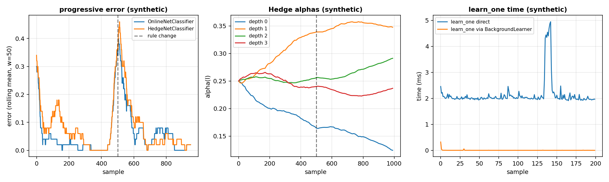
The left panel is the progressive error of OnlineNetClassifier and of HedgeNetClassifier on a synthetic stream of 1000 samples whose rule changes at sample 500 (a vertical dashed line); the rolling mean has window 50. The centre panel is the alphas_ of the Hedge network against the sample. The right panel is the time of learn_one called directly and called through BackgroundLearner on the same estimator: the direct call is around 2 ms, the background call around 0.003 ms.
Details
References
- Sahoo, D., Pham, Q., Lu, J., Hoi, S. C. H. (2018). Online Deep Learning: Learning Deep Neural Networks on the Fly. arXiv:1711.03705. Page 3, Eq.(1):
F(x) = sum_l alpha(l) f(l)(x),f(l) = softmax(h(l) Theta(l)),h(l) = sigma(W(l) h(l-1)),h(0) = x, and the initial weights1 / (L + 1). Page 4, the discountalpha(l) <- alpha(l) beta ** L(f(l)(x), y)withbetain(0, 1)and the loss in(0, 1), the normalisation to sum 1, Eq.(2) forTheta(l)and Eq.(3) forW(l)with the sum fromj = l, the smoothing parametersin(0, 1)that sets a minimum weights / L, and Algorithm 1.
The queue, the worker thread, the snapshot of the served model, the progressive validation and the checkpoint are engineering definitions and carry no citation; the checkpoint is the one of SafeEstimator of the library.
Choices stated explicitly
- A sample is one unit of the learning-rate schedule:
schedule(n_seen_)is the learning rate of the sample numbern_seen_. This is our choice; the schedule is the one of N04, read at the fractional epochepoch + b / n_batchesin the batch training. - The hidden activation of the Hedge network is relu. The paper writes a generic activation
sigma; relu is the one the reference implementation and ourDenselayers use. - The Hedge loss is
1 - p(l)[y]. The paper asks for a value in(0, 1)and does not give the formula; the probability that the classifier gives to the true class is the natural choice, and1 - pis in[0, 1]for a softmax output. - The gradient of every
Theta(l)andW(l)uses the cross-entropy of the classifier, weighted by the currentalpha(l)(Eq.(2) and Eq.(3), page 4). For the multiclass case the loss is the softmax cross-entropy of theDenselayers. - The queue of the
BackgroundLearnerdrops the oldest sample when it is full. This is our choice; the alternative (drop the newest) would lose the most recent data, which on a stream is the part a control loop cares about. - The
served_copy of theBackgroundLearneris made everysync_everyupdates (default 1), in one statement.predict_onereads the copy without waiting for the worker; before the first copy it uses the estimator as it is. - An exception in the worker thread is stored in
error_and raised by the next call oflearn_one,predict_oneorflush, then cleared. The main thread sees it as if it had happened in its own call. budget_sis ten times the measured p99 oflearn_one, never below1e-3:0.06forOnlineNetRegressor(mlp([2, 4, 1]),p99 = 5.94 mson this runtime),0.01forOnlineNetClassifierand forHedgeNetClassifier(bothp99 < 1 ms).memory_classis"O(1)".
Development diary
The delivery leaves out the forgetting of old regimes, gradient clipping and mixed precision: task N07 and N08. The BackgroundLearner uses one worker; more workers would need a different protocol for served_ and are out of this task. The online estimators hold a full copy of the model (model_), so the wrapper and the original share the same Param shapes but are not the same objects; this is the price of the one-copy-per-Param optimizer of N04.