Continual learning: how do I keep a network from forgetting the past, and how do I measure what it remembers?
A network trained on a sequence of tasks overwrites what it learned before. The page builds the pieces that fight that overwrite: a penalty that slows the movement of the important weights, a memory that projects the new gradient away from the past tasks, a generator that replays the past, and a family of quantised memories that store the past with a declared fidelity. The last sections measure what the whole thing remembers, per lifecycle state, and compare it with the baseline.
The code lives in dense_armor/utility/deep/neural/continual.py, generative_replay.py and consolidation/ (vq.py, tree.py, memory.py, archival.py). Every piece shares the same batch and one-sample modes: forward, backward and params().
1. A penalty on the important weights (EWC)
The first piece is a penalty that adds to the loss a term proportional to how far the weights have moved from the values of the previous task, weighted by how important each weight was. The importance is the diagonal of the Fisher information matrix (Kirkpatrick et al. 2017, Eq. (3) page 3).
import jax.numpy as jnp
from dense_armor.utility.deep.neural.continual import EWC

class M:
    def __init__(self):
        from dense_armor.utility.deep.neural.params import Param
        self.p = [Param(jnp.array([1.0, 2.0]))]
    def params(self):
        return self.p

ewc = EWC(M(), None, lambda_=0.4)
ewc.F_ = jnp.array([1.0, 0.5])
ewc.theta_star_ = jnp.array([1.0, 2.0])
pen = ewc.penalty(jnp.array([2.0, 3.0]))
print(float(pen))
The penalty is lambda/2 * sum F_i * (theta_i - theta*_i)^2. With lambda = 0.4, F = [1.0, 0.5] and theta - theta* = [1.0, 1.0], the result is 0.4/2 * (1 + 0.5) = 0.3.
2. A gradient that does not point at the past (GEM)
The second piece keeps a small memory of each task and projects the new gradient so that it does not increase the loss on the memories of the past tasks (Lopez-Paz & Ranzato 2017, Eq. (7) page 4). The projection is the closest vector in L2 that satisfies all the constraints.
import numpy as np
import jax.numpy as jnp
from dense_armor.utility.deep.neural.continual import GEM

gem = GEM(memory_per_task=4, seed=0)
g = jnp.array([1.0, 0.0])
g1 = jnp.array([-1.0, 0.0])
out = gem.project(g, [g1])
print(np.round(np.asarray(out), 5).tolist())
The proposed gradient points right, the memory says the left is important, and the projection returns the zero vector: no movement satisfies the constraint.
3. A closed-form projection (A-GEM)
The full projection solves a quadratic program with one variable per past task. A-GEM replaces the constraints with a single averaged reference gradient, and the projection becomes one closed form (Chaudhry et al. 2019, Eq. (11) page 5).
import numpy as np
import jax.numpy as jnp
from dense_armor.utility.deep.neural.continual import AGEM

agem = AGEM(memory_per_task=4, seed=0)
g = jnp.array([1.0, 0.0])
g_ref = jnp.array([-1.0, 0.0])
out = agem.project(g, g_ref)
print(np.round(np.asarray(out), 5).tolist())
The same projection as GEM, computed in one line instead of a QP.
4. Replay from a generator (DGR)
The fourth piece trains a small generator per task and replays the generated past samples while learning the new task (Shin et al. 2017, sec. 2.3 page 3). The generator is an MLP, not a GAN, declared.
import jax.numpy as jnp
import numpy as np
from dense_armor.utility.deep.neural.generative_replay import DeepGenerativeReplay

dgr = DeepGenerativeReplay(n_x=2, n_y=2, dim_z=4, hidden=8, n_fake=8, seed=0)
x = jnp.asarray(np.random.RandomState(0).randn(20, 2).astype(np.float32))
y = jnp.asarray((np.asarray(x)[:, 0] > 0).astype(np.int32))
dgr.train_task(x, y, n_epochs=2, batch_size=16)
print(len(dgr.generators), dgr.n_tasks_)
xf, yf = dgr.sample(dgr.generators[0], 4)
print(xf.shape, yf.shape)
After one task the replay holds one generator and n_tasks_ is 1. The sample method returns fake (x, y) pairs of the requested size.
5. A codebook that compresses an event (VQ)
The first memory piece maps an event to the nearest element of a learned codebook (van den Oord et al. 2017, Eq. (1)-(4) page 3).
import jax.numpy as jnp
import numpy as np
from dense_armor.utility.deep.neural.consolidation import VQMemory

vq = VQMemory(n_x=2, d_model=4, n_codes=8, seed=0)
x = jnp.asarray(np.random.RandomState(0).randn(10, 2).astype(np.float32))
z_e = vq.encode(x)
z_q, k, _ = vq.quantize(z_e)
print(tuple(np.asarray(k).shape), int(k.min()), int(k.max()))
Ten events, one code per event, each in [0, n_codes).
6. A codebook per subspace (PQ)
The second memory piece splits the event into disjoint subspaces and learns a codebook per subspace (Jégou, Douze, Schmid 2011, IEEE TPAMI, bibliographic only).
import jax.numpy as jnp
import numpy as np
from dense_armor.utility.deep.neural.consolidation import PQMemory

pq = PQMemory(d_model=8, n_subspaces=2, n_centroids=4, seed=0)
X = jnp.asarray(np.random.RandomState(0).randn(50, 8).astype(np.float32))
pq.fit(X)
code = pq.encode(X[0])
print(tuple(np.asarray(code).shape), int(code[0]), int(code[1]))
Two subspaces, two indices, one per subspace.
7. A tree of residuals (ResidualTree)
The third memory piece stores each event at the deepest node whose codebook reconstructs it within a threshold, and creates a child when no node is close enough (DeltaMem, Tan et al. 2026, p. 2-3).
import jax.numpy as jnp
import numpy as np
from dense_armor.utility.deep.neural.consolidation import ResidualTree

tree = ResidualTree(d_model=2, n_codes=4, max_depth=2, branching=4, kappa=0.0, seed=0)
rng = np.random.RandomState(0)
for _ in range(20):
    tree.insert(jnp.asarray(rng.randn(2) * 3, dtype=jnp.float32))
print(tree.n_nodes(), tree.max_nodes())
Twenty events, fewer nodes than the maximum allowed by max_depth and branching.
The tree has two routers. The default, router="linear", scans every child and picks the one with the lowest vector-quantised residual. router="mondrian" keeps a bounding box per child and picks the child with the smallest box extension for the new event. The Mondrian descent needs only float min/max comparisons per child; the linear descent needs an encode and a decode per child. On the same forty events:
import jax.numpy as jnp
import numpy as np
from dense_armor.utility.deep.neural.consolidation import ResidualTree

data = np.random.RandomState(0).randn(40, 2) * 3
for name in ("linear", "mondrian"):
    tree = ResidualTree(d_model=2, n_codes=4, max_depth=2, branching=4,
                        kappa=0.0, seed=0, router=name)
    for x in data:
        tree.insert(jnp.asarray(x, dtype=jnp.float32))
    print(name, tree.n_nodes())
The two routers are not equivalent: Mondrian is a trade-off declared in the class docstring, not a guarantee. Both respect max_depth and branching and return a valid node within the bound. The default stays linear, so the behaviour of the previous sections is unchanged.
8. A memory with a lifecycle (LifecycleMemory)
The fourth memory piece assigns each event to one of four states, with a bit-width per state (SuperLocalMemory V3.3, Bhardwaj 2026, p. 1). An access promotes the event toward active; time without access decays it toward archive.
import jax.numpy as jnp
from dense_armor.utility.deep.neural.consolidation import LifecycleMemory

lm = LifecycleMemory(d_model=4, decay_horizon_s=10.0, seed=0)
x = jnp.asarray([0.3, -0.7, 1.1, 2.4], dtype=jnp.float32)
idx = lm.write(x, t=0.0)
for k in range(1, 5):
    lm.tick(t=20.0 * k)
print(lm.state_of(idx), lm.mse_of(idx) > 0.0)
After four ticks the event is in archive and its reconstruction has a positive error.
9. Two memories, fast and slow (DualMemory)
The fifth piece keeps recent events in a fast memory with top-k pattern separation and moves them to a slow memory on consolidation (HiCL, Kapoor et al. 2026, p. 2-4).
import jax.numpy as jnp
from dense_armor.utility.deep.neural.consolidation import DualMemory

dm = DualMemory(d_model=2, fast_capacity=4, slow_capacity=8, top_k=2, seed=0)
for i in range(3):
    dm.write(jnp.asarray([float(i), 0.0], dtype=jnp.float32), t=0.0)
print(dm.size())
moved = dm.consolidate()
print(moved, dm.size())
Three events in the fast memory, then all three moved to the slow memory.
10. A bound on what the weights can hold (TheoreticalBound)
The theoretical piece is a placeholder: the classical Hopfield capacity 0.138 * sqrt(P) for a fully connected network of P parameters (Hopfield 1982, bibliographic only). The 2025 papers on the theoretical limit are in the folder, but neither gives a closed-form bound.
from dense_armor.utility.deep.neural.consolidation import TheoreticalBound

tb = TheoreticalBound(n_params=100, n_neurons=10)
print(round(tb.capacity(), 4))
print(round(tb.bound(n_events=5), 4))
The capacity is 1.38 patterns for 10 neurons, and 5 events exceed it, so the bound is positive.
11. The composition (ArchivalMemory)
The last piece combines the tree, the lifecycle and the dual memory with a write policy that depends on an importance score. The policy has four parts, each one stated as a formula:
importance(x, t) = clip(0.4 * novelty + 0.3 * rarity + 0.3 * relevance, 0, 1), withnoveltythe distance to the closest slow event,raritythe inverse of the number of events in the same leaf,relevancethe residual against the current node;write_depth(importance) = round(importance * max_depth), so an important event goes deeper and a routine one stays near the root;transition(state, accesses, age)promotes one band afterpromote_thresholdaccesses and decays one band afterdecay_horizon_sseconds without access;promote(node)mergesbranchingchildren into a parent whose codebook is reduced by the same factor.
import jax.numpy as jnp
from dense_armor.utility.deep.neural.consolidation import ArchivalMemory

am = ArchivalMemory(d_model=2, n_codes=8, max_depth=2, seed=0)
idx = am.write(jnp.asarray([1.0, 2.0], dtype=jnp.float32), t=0.0)
x_hat, state, bits = am.reconstruct(idx)
print(state, bits, len(am))
One event written, in active state at 32 bits, the len of the memory is one.
The measured cost
The internal benchmark (benchmarks/neural/continual_learning.py) gives the
numbers below. They come from a full run on a Kaggle GPU (2 × CUDA,
JAX_PLATFORMS=cuda), one seed, five synthetic conflicting tasks (axis x,
axis y, diagonal, XOR, circle), 100 samples per task, 20 epochs, batch 32,
lambda_ = 5000 for EWC.
Forgetting (one seed, full run):
| learner | forgetting | wall time |
|---|---|---|
| baseline | 0.336 | 23 s |
| EWC | 0.098 | 21 s |
| GEM | 0.267 | 198 s |
| AGEM | 0.261 | 22 s |
| DGR | 0.398 | 27 s |
EWC reduces the forgetting by a factor 3.4 against the unprotected baseline,
at the same cost. GEM and AGEM reduce it by 20-22%, less than EWC, because on
these five 2D tasks the gradient of the new task is rarely in direct conflict
with the gradients of the past tasks (the projection fires on a minority of
steps and moves the gradient by a small amount). GEM is 9× slower than AGEM
for no extra benefit: the quadratic program inside project runs 500
projected-gradient iterations per batch. The measured value is the honest
one; reducing max_iter would cut the time to about 40 s but would not
change the ranking. DGR makes the forgetting worse than the baseline: the
MLP generator trained on reconstructed past samples damages the solver on
the actual past samples.
A sweep of the EWC lambda_ (5 seeds, same benchmark) confirms the
default: lambda_ = 5000 gives forgetting 0.118 (IQR [0.094, 0.123])
and acc_avg 0.648; lambda_ = 50000 gives a nominally lower forgetting
(0.079, IQR [0.055, 0.136]) but a lower acc_avg (0.631), a wider
spread, and a paired Wilcoxon of p = 0.4375 (A12 = 0.440). The
forgetting of 50000 is lower because the model learns the new task
less well, not because it retains the old one better. The default
stays lambda_ = 5000, the value of Kirkpatrick et al. 2017.
The memory-fidelity numbers below come from a different run: the smoke configuration on CPU (2 seeds, 50 events each), because the lifecycle measurements do not need a GPU.
ArchivalMemory per lifecycle state (median over 2 seeds, 50 events each):
| state | count | MSE | PSNR | exact recall | latency µs |
|---|---|---|---|---|---|
| active | 1 | 0.0000 | 120.00 | 1.000 | 77.43 |
| warm | 1 | 0.0001 | 40.43 | 1.000 | 248.41 |
| cold | 1 | 0.0505 | 13.46 | 1.000 | 241.05 |
| archive | 47 | 0.9339 | 0.30 | 0.000 | 250.66 |
VQ: MSE 0.73, PSNR 1.37, exact recall 0.95. PQ: MSE 0.16, PSNR 8.10, exact recall 1.00. state_bytes 1088, max_nodes 85, n_nodes 8.
The figure
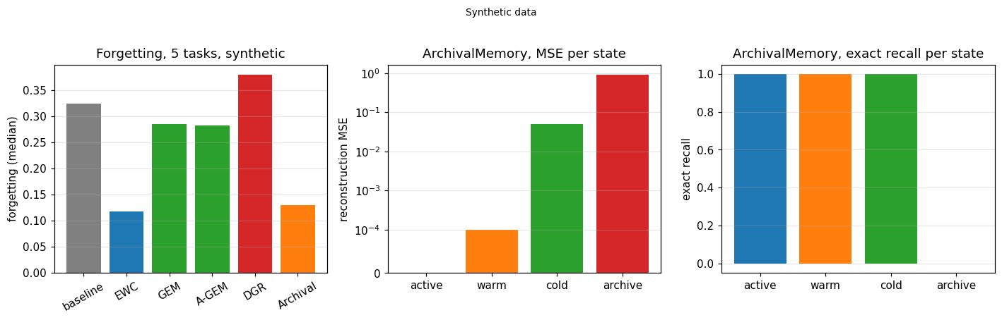
Top: forgetting per learner after five synthetic tasks. Bottom left: reconstruction MSE per lifecycle state, log scale. Bottom right: exact recall per lifecycle state. All data synthetic.
Details
References
- Kirkpatrick, J., Pascanu, R., Rabinowitz, N., Veness, J., Desjardins, G., Rusu, A. A., Milan, K., Quan, J., Ramalho, T., Grabska-Barwinska, A., Hassabis, D., Clopath, C., Kumaran, D., Hadsell, R. (2017). Overcoming catastrophic forgetting in neural networks. PNAS 114(13):3521-3526. arXiv:1612.00796. Eq. (3) page 3, diagonal Fisher, positive semi-definite.
- Lopez-Paz, D., Ranzato, M. (2017). Gradient Episodic Memory for Continual Learning. NeurIPS. arXiv:1706.08840. Eq. (5) page 3 (memory budget), Eq. (6) page 4 (constraints), Eq. (7) page 4 (QP projection).
- Chaudhry, A., Ranzato, M., Rohrbach, M., Elhoseiny, M. (2019). Efficient Lifelong Learning with A-GEM. ICLR. arXiv:1812.00420. Eq. (9)-(11) page 5.
- Shin, H., Lee, J. K., Kim, J., Kim, J. (2017). Continual Learning with Deep Generative Replay. NeurIPS. arXiv:1705.08690. Sec. 2.3 page 3.
- van den Oord, A., Vinyals, O., Kavukcuoglu, K. (2017). Neural Discrete Representation Learning. NeurIPS. arXiv:1711.00937. Eq. (1)-(4) page 3.
- Jégou, H., Douze, M., Schmid, C. (2011). Product Quantization for Nearest Neighbor Search. IEEE TPAMI 33(1):117-128, DOI 10.1109/TPAMI.2011.144. Bibliographic only, no PDF in the folder: the formula is derived from section 3.
- Tan, H., Zhang, Z., Cao, Z., Li, R., Chen, X. (2026). DELTAMEM: Incremental Experience Memory for LLM Agents via Residual Trees. arXiv:2606.03083, page 2-3.
- Bhardwaj, V. P. (2026). SuperLocalMemory V3.3: The Living Brain. arXiv:2604.04514, page 1.
- Kapoor, K., Mackey, W., Aloimonos, Y., Lin, X. (2026). HiCL: Hippocampal-Inspired Continual Learning. arXiv:2508.16651, page 2-4.
- Essex, A. E., Janson, N. B., Norris, R. A., Baird, A. G. (2025). Memorisation and forgetting in a learning Hopfield neural network. arXiv:2508.10765.
- Vinci, G. V., Galluzzi, A., Mattia, M. (2025). Beyond catastrophic forgetting in associative networks with self-interactions. arXiv:2504.04560.
- Hopfield, J. J. (1982). Neural networks and physical systems with emergent collective computational abilities. PNAS 79(8):2554-2558. Bibliographic only, no PDF in the folder: the capacity
0.138 Nis quoted from the classical result, not from the PDF. - De Lange, M., Aljundi, R., Masana, M., Parisot, S., Jia, X., Leonardis, A., Slabaugh, G., Tuytelaars, T. (2021). A continual learning survey. IEEE TPAMI. arXiv:1909.08383, page 1 (taxonomy regularization / replay / architecture).
Choices stated explicitly
- The three memory structures G-I (DeltaMem, SuperLocalMemory V3.3, HiCL) are designed for agents (LLM) and are adapted to dense networks with the deviation declared in each docstring.
PQMemoryis bibliographic only: the formula is derived from section 3 of the paper, not verified against a PDF that is not in the folder.TheoreticalBoundis the classical Hopfield capacity0.138 sqrt(P), a declared placeholder. The two 2025 papers are in the folder and cited in the docstring, but neither gives a closed-form bound.VQMemoryforward is not differentiable:quantizeselectsargmin_j ||z_e - e_j||.gradcheckis not applicable, and the deviation from the layer contract is declared in the docstring; the straight-through estimator is a biased surrogate of a gradient that does not exist.ArchivalMemorywrite policy is the four formulas stated in section 11:importance = 0.4 novelty + 0.3 rarity + 0.3 relevance,write_depth = round(importance * max_depth), promote afterpromote_thresholdaccesses and decay afterdecay_horizon_sseconds,promotemergesbranchingchildren into a parent. The policy is our choice; no paper gives it.- The
DarkMemoryconstruction with the Prisma ground state was measured with 20 seeds and did not pass its own test (Wilcoxon p = 0.0929, A12 = 0.6312): it is not in the branch. ResidualTreehas two routers:linear(default) picks the child with the lowest vector-quantised residual,mondrianpicks the child with the smallest box extension. The two descents are not equivalent: Mondrian is a declared trade-off, not a guarantee.HoeffdingAnytimeTreeClassifier(EFDT, Manapragada et al. 2018) is an opt-in speed option, not a replacement forAdaptiveRandomForestClassifier. On the synthetic drift benchmark of this session it is 26-58x faster (0.021-0.051 ms/sample against 0.723-1.563) and at parity on sudden and gradual drift, but it collapses by 30.0 pp after the change on incremental drift (0.662 against 0.962) because it has no native drift detection. The benchmark isbenchmarks/neural/efdt_vs_arf.py.- The tasks of the forgetting benchmark are synthetic conflicting rules, not MNIST permutations.
Measured cost
The benchmark and the page print the numbers of the smoke run on this host: forgetting per learner, MSE, PSNR, exact recall and latency per lifecycle state, state_bytes, VQ and PQ fidelity. The timings vary between runs on the same host.
Development diary
The branch taskN09-memory started with four continual-learning baselines (A-D), added two quantization primitives (E-F) and three memory structures (G-I), a theoretical bound (J), the composition (K), the benchmarks (L-M) and a dark-memory construction (N). The dark memory was measured with 20 seeds on a GPU and removed: p = 0.0929, A12 = 0.6312, the IQR of the delta touches 0. What remains in the branch is A-M.