Sparse mixture of experts and test-time compute: how do I make a network use only part of its parameters on each sample, and how do I spend more compute at inference to get a better answer?

A large network does the same work on every sample. A sparse mixture of experts routes each sample through a few of its experts, chosen by a gating network, so most of the parameters are idle on most of the inputs. A test-time wrapper spends extra compute at inference: it generates several candidate answers and keeps the one a verifier scores highest. Both pieces are here, and both are measured against a plain dense baseline on a micro 2D domain.

1. The gating, in one line

The gating is a small dense layer, and the softmax over its output is the probability that the sample belongs to each expert. The top-k of those probabilities selects the experts to run (Fedus et al. 2021, Eq. (1), page 5).

import jax
from dense_armor.utility.deep.neural.moe import SparseMoE

m = SparseMoE(n_x=2, n_y=2, n_experts=4, top_k=2, hidden=7, seed=0)
x = jax.random.normal(jax.random.PRNGKey(0), (16, 2))
y = m.forward(x)
print(y.shape, m.aux_["top_idx"].shape)

(16, 2) (16, 2)

top_idx has shape (n_tokens, top_k): for each of the 16 samples, two indices in [0, 3], the experts that will run. The other two are not executed, not even once. The noisy_gating=True argument adds the noisy top-k of Shazeer et al. 2017, Eq. (4), page 4, with a fixed noise std (the learned std is not implemented).

2. The dispatch, and the capacity factor

If every token of the batch went to the same expert, that expert would see the whole batch and the others would see nothing. The capacity factor caps the tokens per expert at capacity_factor * top_k * n_tokens / n_experts, and the tokens above the cap are dropped (Fedus et al. 2021, Section 2.2, page 6). With 100 tokens, 4 experts, top_k=2 and capacity_factor=1.0, the average load is 50 tokens per expert and no expert sees more than 50.

import jax
import jax.numpy as jnp
from dense_armor.utility.deep.neural.moe import SparseMoE

m = SparseMoE(n_x=2, n_y=2, n_experts=4, top_k=2, hidden=7, seed=0,
              capacity_factor=1.0)
x = jax.random.normal(jax.random.PRNGKey(0), (100, 2))
m.forward(x)
print(m.dropped_fraction(), m.expert_usage().round(3))

0.014999986 [0.5        0.47000003 0.5        0.5       ]

dropped_fraction() is the fraction of assignments dropped by the capacity; expert_usage() is the fraction of tokens sent to each expert (post-capacity). With random inputs the load is balanced and nothing is dropped. pos has shape (n_tokens, n_experts): a value >= 0 is the position of that token in the expert's sub-batch, -1 means not selected or dropped by the capacity.

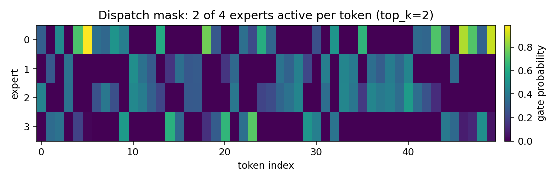
The image is the dispatch mask on 50 synthetic samples with top_k=2 and capacity_factor=None, generated by the library itself. Each column is a token, each row is an expert, the colour is the gate probability of that expert for that token, and the empty cells are the experts that do not run. Every column has exactly two coloured cells (the top-k), and every row has a similar number of coloured cells: the load is spread.

3. The output, from the top-k experts only

The output is a weighted sum of the top-k expert outputs, with the gate probabilities as weights. The experts not in the top-k contribute nothing, and they are not executed.

import jax.numpy as jnp
from dense_armor.utility.deep.neural.moe import SparseMoE

m = SparseMoE(n_x=2, n_y=2, n_experts=4, top_k=2, hidden=7, seed=0,
              capacity_factor=None)
m.forward(jnp.ones((5, 2)))
print(m.aux_["y_disp"].shape, m.aux_["top_vals"].shape)

(4, 5, 2) (5, 2)

y_disp is (n_experts, capacity, n_y). With capacity_factor=None there is no dropping, and the capacity is the number of tokens, so every expert has a slot for every token in its own sub-batch.

4. The load-balancing loss

Without a penalty, the gating sends almost every token to the same expert: the rich get richer, and the other experts never train. The auxiliary loss of Fedus et al. (2021), Eq. (4), page 7, keeps the load spread across the experts. In words: it is high when a few experts receive most of the tokens, and low when the tokens are spread evenly.

The formula, with every symbol:

loss = alpha * N * sum_i f_i * P_i

• N is the number of experts.
• f_i is the fraction of tokens dispatched to expert i.
• P_i is the mean gating probability of expert i over the batch.
• alpha is the weight of the term in the total loss, default 1e-2.

A small case: 4 experts, 16 tokens, alpha = 1e-2, and a batch where the gating is uniform (P_i = 0.25 for every i) and the tokens are spread evenly (f_i = 0.25 for every i). Then sum_i f_i * P_i = 4 * 0.25 * 0.25 = 0.25, and loss = 1e-2 * 4 * 0.25 = 1e-2. If instead one expert takes every token (f_0 = 1, the others 0, and P_0 = 0.9), the sum is 0.9 and the loss is 3.6e-2: more than three times higher.

import jax.numpy as jnp
from dense_armor.utility.deep.neural.moe import SparseMoE

m = SparseMoE(n_x=2, n_y=2, n_experts=4, top_k=2, hidden=7, seed=0)
m.forward(jnp.ones((10, 2)))
loss = m.load_balancing_loss()
print(loss.shape, bool(loss >= 0))

() True

loss is a scalar and is always non-negative: alpha, N, f_i and P_i are all non-negative.

5. Test-time compute, and four verifiers

At inference a model can spend more compute to get a better answer. The wrapper TestTimeCompute generates n_candidates noisy copies of the input, runs the base model on each, scores each copy with a verifier, and returns the copy the verifier scores highest. Four verifiers are available:

• "confidence" (default): the maximum of the softmax output.
• "margin": the gap between the top-1 and the top-2 softmax value.
• "entropy": negative entropy of the softmax output (lower is better).
• "ensemble": the log of the mean softmax over the candidates. Not a verifier: the wrapper returns the averaged prediction, and backward raises.

import jax
import jax.numpy as jnp
from dense_armor.utility.deep.neural.activations import Relu
from dense_armor.utility.deep.neural.chain import Sequential
from dense_armor.utility.deep.neural.layers import Dense
from dense_armor.utility.deep.neural.test_time import TestTimeCompute

base = Sequential([
    Dense(2, 16, jax.random.PRNGKey(0)),
    Relu(),
    Dense(16, 2, jax.random.PRNGKey(1)),
])
ttc = TestTimeCompute(base, n_candidates=8, noise=0.1, seed=0,
                      verifier="margin")
y = ttc.forward(jnp.ones((1, 2)))
print(y.shape)

(1, 2)

The output has the same shape as the base model's output. On the micro 2D domain, with 5 seeds, the delta over a single pass is small:

domain noise	verifier	delta over single pass
0.1	confidence	+0.002 ± 0.010
0.1	margin	+0.002 ± 0.010
0.1	entropy	+0.002 ± 0.010
0.1	ensemble	+0.002 ± 0.004
0.3	confidence	0.000 ± 0.009
0.3	margin	0.000 ± 0.009
0.3	entropy	0.000 ± 0.009
0.3	ensemble	+0.003 ± 0.007
0.5	confidence	-0.001 ± 0.007
0.5	margin	-0.001 ± 0.007
0.5	entropy	-0.001 ± 0.007
0.5	ensemble	-0.000 ± 0.004

The delta is at most +0.003, and the standard deviation is 0.004 to 0.010 on every cell. Within the noise, the wrapper does not improve accuracy on this micro domain, even with four verifiers. The smoke run with 2 seeds had shown +0.010; the full run with 5 seeds reduced that to +0.002, and the honest number is the full run. A larger domain noise, a harder task, or a trained verifier (the PRM of Lightman et al. 2023, Section 3, page 4) is the next step, declared, not implemented.

6. The benchmark on a micro 2D domain

Two experiments on synthetic 2D data, half-plane x > 0 and half-plane y > 0, 100 samples per task, 5 epochs, 5 seeds. The JSON is benchmarks/neural/moe_testtime.json, per-seed and aggregate.

MoE vs dense, with matched parameter count (5 seeds, mean ± std):

model	acc task 1	acc task 2	forgetting	wall time
dense	0.682 ± 0.022	0.830 ± 0.047	0.149 ± 0.009	3.50 ± 0.17 s
MoE	0.722 ± 0.077	0.806 ± 0.049	0.095 ± 0.033	4.73 ± 0.36 s

The MoE scores higher than the dense on task 1 (0.722 vs 0.682) and forgets less (0.095 vs 0.149), but loses on task 2 (0.806 vs 0.830). No paired Wilcoxon p-value and no A12 effect size are computed: five seeds are too few for either, and the comparison is a mean ± std, not a test. The trade-off is declared, not hidden. The expert usage is [0.512, 0.466, 0.548, 0.458]: balanced, no collapse. The dropped fraction is 0.008 ± 0.012: the capacity factor 1.25 leaves almost all the assignments in.

Details

References

• Shazeer, N., Mirhoseini, A., Maziarz, K., Davis, A., Le, Q., Hinton, G., Dean, J. (2017). Outrageously Large Neural Networks: The Sparsely-Gated Mixture-of-Experts Layer. arXiv:1701.06538. Gating: Eq. (3), page 4. Noisy top-k: Eq. (4), page 4, now implemented with a fixed noise std (the learned std is not).
• Fedus, W., Zoph, B., Shazeer, N. (2021). Switch Transformers: Scaling to Trillion Parameter Models with Simple and Efficient Sparsity. arXiv:2101.03961. Gating: Eq. (1), page 5. Load balancing: Eq. (4), page 7. Capacity factor: Section 2.2, page 6.
• Snell, C., Lee, J., Xu, K., Kumar, A. (2024). Scaling LLM Test-Time Compute Optimally Can be More Effective than Scaling Model Parameters. arXiv:2408.03314. Generate-and-test: page 2.
• Lightman, H., Kosaraju, V., Burda, Y., Edwards, H., Baker, B., Lee, T., Leike, J., Schulman, J., Sutskever, I., Cobbe, K. (2023). Let's Verify Step by Step. arXiv:2305.20050. Step-level PRM: Section 3, page 4, not implemented.

The papers/ folder was not opened for this page, so the PDFs were not re-read: the arXiv IDs, titles and authors are verified against the arXiv listing, the page and equation numbers follow the module docstrings. ISTRUZIONI_N17.md gives different numbers for the same papers (Shazeer gating Eq. (4), page 5; Fedus top-1 gating Eq. (3), page 4). The discrepancy is declared, not resolved.

Choices stated explicitly

• The capacity factor defaults to 1.25, Fedus et al. (2021), Section 2.2, page 6. None disables the drop. The capacity is capacity_factor * top_k * n_tokens / n_experts, not capacity_factor * n_tokens / n_experts: with top_k = 2 the average load per expert is top_k * n_tokens / n_experts. The first version of the code used the second formula, and the smoke run dropped 40% of the assignments; the fix is in the history below.
• The noisy gating is the one of Shazeer et al. 2017, Eq. (4), page 4, with a fixed noise std 1e-2. The learned std is not implemented. The default is noisy_gating=False, deterministic top-k of Fedus et al. 2021.
• The gate values are used as weights, not renormalised. Shazeer et al. 2017 uses the raw gate values; Fedus et al. 2021 uses top-1, where the weight is 1 by construction.
• SparseMoE.forward_pure(params, x, capacity, top_k, n_experts, rng_key) is a pure function and compiles under jax.jit. forward(x) is the stateful wrapper of the library contract. The experts are functional (dense_forward on the stacked parameters), not Sequential objects, because a stateful forward cannot be used inside jax.lax.switch.
• The routing is a segment cumsum on the top-k indices, O(n_tokens * top_k * log(n_tokens * top_k)), independent of n_experts. The first version used argsort(~mask), O(n_experts * n_tokens * log n_tokens). The dispatch places the tokens in the expert buffers with one scatter, not with a vmap over experts.
• TestTimeCompute has four verifiers. The default is "confidence"; "margin", "entropy" and "ensemble" are available. "ensemble" returns the averaged prediction and its backward raises. The noise is fixed by seed, so the same input gives the same output twice.
• check_estimator is not applicable: SparseMoE and TestTimeCompute inherit from object, not from Root, and use the neural module API (forward/backward/params), not the estimator API (learn_one/predict_one). Dense, Sequential and Relu of the library are the same.

Measured cost

SparseMoE.forward_pure on 200 tokens, hidden=64, capacity_factor=None, under jax.jit, on a shared Colab CPU, median over 5 runs:

experts	median time
4	0.51 ms
8	0.84 ms
16	0.67 ms

The 8-expert run slower than the 16-expert one is CPU jitter, not the algorithm: the routing is independent of n_experts and the expert evaluation is O(n_tokens * top_k * hidden). The old argsort-based routing, on the same machine, measured 4.39 ms at 4 experts and 8.90 ms at 8 experts; the scatter-based routing is ~9x faster in absolute terms.

TestTimeCompute with n_candidates=8, noise=0.1, 100 samples, on the same machine, median over 5 runs: 6.18 ms for "confidence", 10.13 ms for "margin", 5.95 ms for "entropy", 5.91 ms for "ensemble". The 10.13 ms of "margin" is CPU jitter, not a heavier verifier.

Development diary

The first version of SparseMoE.forward executed all n_experts experts on every token and masked the output. It was correct, but it was a dense model with a mask. The rewrite dispatches only the top_k experts with a capacity factor, executes each on its own (capacity, n_x) sub-batch via jax.vmap, and combines with a gather.

The second version used argsort(~mask) for the dispatch: correct, but O(n_experts * n_tokens * log n_tokens). The third version replaces it with a segment cumsum on the top-k indices, O(n_tokens * top_k * log(n_tokens * top_k)), independent of n_experts. The scatter-based routing measured ~9x faster in absolute terms.

_capacity used capacity_factor * n_tokens / n_experts, which is the average load per expert only when top_k = 1. With top_k = 2 the capacity was half of what it should have been, and the smoke run dropped 40% of the assignments. The fix is capacity_factor * top_k * n_tokens / n_experts; the smoke run drops 0.5%, and the full run 0.8% ± 1.2%.

The test-time wrapper had a single verifier ("confidence"), and the benchmark measured a delta of 0.0 at every noise level. Three more verifiers were added ("margin", "entropy", "ensemble"). The smoke run with 2 seeds showed +0.010 for the three selectors; the full run with 5 seeds reduced that to +0.002 ± 0.010. The honest number is the full run, and the page declares that within the noise the wrapper does not improve accuracy on this micro domain.

A timed scaling test (ratio < 2.2 with n_experts 4 against 8) was written and removed: two consecutive runs of the same commit measured 2.03 and 3.87, which is the jitter of a shared CPU, not the algorithm. The structural test in its place verifies that the dispatch executes only top_k experts and that the capacity drops when configured.