Graph and spectrum
A signal on a graph can change slowly from node to node or fast. The spectrum of the graph tells you which is which. This page builds a graph, finds its frequencies and moves a signal into them and back.
1. A graph and its Laplacian
Graph(n, edges) is a weighted graph with nodes 0 .. n-1 and edges (i, j, w). Its Laplacian L = D - W has the degree of each node on the diagonal and minus the weight of each edge off it (Niresi and others 2024, Eq. 1).
from dense_armor.core.graph import Graph

g = Graph(4, [(0, 1, 1.0), (1, 2, 1.0), (2, 3, 1.0)])
print(g.n_nodes, g.n_edges, g.degrees.tolist())
print(g.laplacian.toarray().astype(int).tolist())
The graph is a path of four nodes. The two ends have one neighbour, so their degree is 1; the two middle nodes have two. A bad node index, a self-loop, a repeated pair or a weight that is not positive and finite raises ValueError. g.normalized_laplacian is I - D^(-1/2) W D^(-1/2); a node with no edge has a row and a column of zeros, the convention of NetworkX.
2. The frequencies of the graph
The eigenvalues of L are the frequencies and its eigenvectors are the patterns that go with them. eigendecomposition(L) returns both, the eigenvalues in ascending order.
from dense_armor.core.graph import Graph, eigendecomposition, fiedler_vector

g = Graph(4, [(0, 1, 1.0), (1, 2, 1.0), (2, 3, 1.0)])
w, U = eigendecomposition(g.laplacian)
print(abs(w).round(4).tolist())
print(fiedler_vector(g.laplacian).round(4).tolist())
The first eigenvalue is 0 and goes with a constant pattern: no change from node to node. The larger the eigenvalue, the faster the pattern changes along the edges. The second eigenvector is the Fiedler vector: it has one sign change, and it splits the path in the middle.
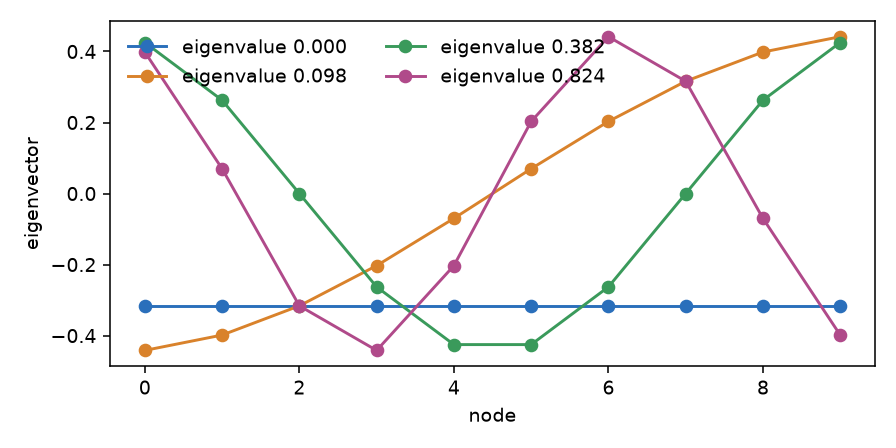
The four lowest patterns of a path of ten nodes. The eigenvalue 0 is a flat line; each next one crosses zero once more.
The decomposition is dense (numpy.linalg.eigh): time grows as n^3 and memory as n^2. For a large graph use the Chebyshev filter, which does not need it. On a graph that is not connected the second eigenvalue is 0 and its eigenvector is not unique.
3. A signal in frequencies, and back
gft(x, U) writes the signal x as a sum of the patterns: it gives U^T x (Liu and others 2024, Section 2). igft goes back.
import numpy as np
from dense_armor.core.graph import Graph, eigendecomposition, gft, igft

g = Graph(4, [(0, 1, 1.0), (1, 2, 1.0), (2, 3, 1.0)])
w, U = eigendecomposition(g.laplacian)
x = np.array([1.0, 2.0, 3.0, 4.0])
xh = gft(x, U)
print(np.abs(xh).round(4).tolist(), np.allclose(igft(xh, U), x), round(float(x @ x), 4), round(float(xh @ xh), 4))
The signal rises by one at every node, so it sits almost entirely in the first two frequencies. The sign of each number depends on the sign of its eigenvector, which is arbitrary; fix_sign(U) makes it fixed. The transform keeps the energy (30 and 30, the Parseval relation) and igft returns the signal.
The numbers are shown in absolute value because the sign of each one depends on the sign of its eigenvector.
4. The same transform as an object
When you transform many signals on the same graph, find the basis once. GraphFourier(graph) does the decomposition when it is created and keeps the frequencies and the basis.
from dense_armor.core.graph import Graph, GraphFourier

g = Graph(4, [(0, 1, 1.0), (1, 2, 1.0), (2, 3, 1.0)])
f = GraphFourier(g)
print(abs(f.eigenvalues).round(4).tolist())
print(abs(f.transform([1.0, 2.0, 3.0, 4.0])).round(4).tolist())
f.eigenvalues are the frequencies, f.basis holds the patterns as columns, f.transform(x) is U^T x and f.inverse(x_hat) goes back. GraphFourier(g, normalized=True) uses the normalised Laplacian, whose frequencies lie in [0, 2].
5. A signal that knows its graph
GraphSignal(signal, graph) joins a Signal with one channel per node to the graph. values is the array of the channels in the order of signal.names; a signal with a different number of channels raises ValueError.
from dense_armor.core.graph import Graph, GraphSignal
from dense_armor.roles import Signal

g = Graph(3, [(0, 1, 1.0), (1, 2, 1.0)])
s = Signal([1.0, 2.0, 4.0], names=["a", "b", "c"], units=["", "", ""])
gs = GraphSignal(s, g)
print(gs.n_nodes, gs.values.tolist(), gs.to_signal() is s)
Details
The library has no function that builds a graph from data: the edges are yours. to_networkx() and to_pygsp() hand the same weights to those libraries. fix_sign flips each column so that its first entry above 1e-9 is positive. The tests compare gft with PyGSP on the absolute value, because the two libraries do not choose the same sign. The paper of the transform (Liu and others 2024, Section 2) takes the eigenvectors of the normalised Laplacian, whose eigenvalues lie in [0, 2]; gft accepts the eigenvectors of any symmetric Laplacian, so eigendecomposition(g.normalized_laplacian) gives the paper's basis and eigendecomposition(g.laplacian) the combinatorial one used on this page. g.laplacian is a CSR sparse matrix, so g.laplacian[0, 0] works.